Simple linear regression
Definition taught in Linear regression, part of Statistical inference
Simple linear regression
| Type | Definition |
| Taught in | Linear regression |
| Part | Statistical inference |
| Properties | 3 |
| Worked examples | 2 |
The simple linear regression model says
Y_i=\beta_0+\beta_1 x_i+\varepsilon_i, \qquad \varepsilon_i\ \text{independent}\ \operatorname{N}(0,\sigma^2),
with the x_i treated as fixed and not all equal. Equivalently, the Y_i are independent and Y_i\sim\operatorname{N}(\beta_0+\beta_1 x_i,\sigma^2).
Properties
Least-squares estimators are unbiased
Main article: Least-squares estimators are unbiased
If \mathbb{E} Y_i=\beta_0+\beta_1x_i for every i, then \mathbb{E}\widehat\beta_1=\beta_1 and \mathbb{E}\widehat\beta_0=\beta_0. No assumption about the error distribution is needed.
Sampling distribution of the regression estimators
Main article: Sampling distribution of the regression estimators
Under simple linear regression,
\widehat\beta_1\sim\operatorname{N}\Bigl(\beta_1,\ \frac{\sigma^2}{S_{xx}}\Bigr), \qquad \widehat\beta_0\sim\operatorname{N}\Bigl(\beta_0,\ \frac{\sigma^2\sum_ix_i^2}{nS_{xx}}\Bigr),
and with S^2=\frac1{n-2}\sum(Y_i-\widehat\beta_0-\widehat\beta_1x_i)^2,
\frac{(n-2)S^2}{\sigma^2}\sim\chi^2_{n-2},
independently of (\widehat\beta_0,\widehat\beta_1). In particular S^2 is unbiased for \sigma^2. Moreover \widehat\beta_1 and \overline Y are independent.
Slope t pivot
Main article: Slope t pivot
Under simple linear regression,
\frac{\widehat\beta_1-\beta_1}{S_1}=\frac{\widehat\beta_1-\beta_1}{S/\sqrt{S_{xx}}}
has the t_{n-2} distribution.
Examples
Heart rate and oxygen intake
Worked example from Linear regression
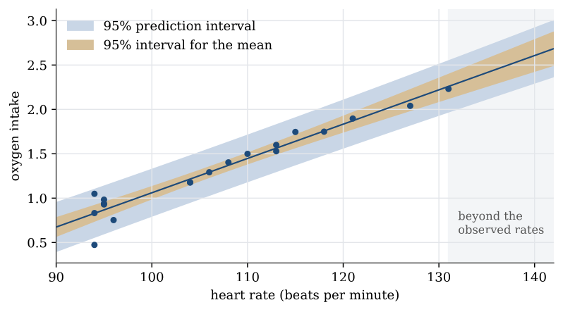
For one person, heart rate and oxygen intake are measured together 19 times.
| Heart rate | 94 | 96 | 95 | 95 | 94 | 95 | 94 | 104 | 104 | 106 |
|---|---|---|---|---|---|---|---|---|---|---|
| Oxygen | 0.473 | 0.753 | 0.929 | 0.939 | 0.832 | 0.983 | 1.049 | 1.178 | 1.176 | 1.292 |
| Heart rate | 108 | 110 | 113 | 113 | 118 | 115 | 121 | 127 | 131 |
|---|---|---|---|---|---|---|---|---|---|
| Oxygen | 1.403 | 1.499 | 1.529 | 1.599 | 1.749 | 1.746 | 1.897 | 2.040 | 2.231 |
Question. Fit the regression of oxygen intake on heart rate, give a 95% interval for the slope, and test whether the slope is zero.
Solution. Here \overline x=107.0 and S_{xx}=2518. The fitted line is y=-2.804+0.03865\,x. The residual standard deviation is S=0.1205, so S_1=0.1205/\sqrt{2518}=0.00240 and S_0=0.258. With t_{17;0.975}=2.110, the 95% interval for the slope is
0.03865\pm2.110\times0.00240=(0.0336,\ 0.0437).
It excludes zero. Equivalently, t=0.03865/0.00240=16.1, far beyond 2.110, so H_0:\beta_1=0 is rejected. Each extra beat per minute goes with about 0.039 more units of oxygen.
Height and shoe size
Worked example from Regression examples
Question. Fit the regression of height on shoe size and interpret the output.
Solution.
survey <- read.csv("studentsurvey.csv")
model1 <- lm(height ~ shoe, data = survey)
summary(model1)
# Residuals:
#      Min       1Q   Median       3Q      Max
# -18.9073  -6.1465   0.1096   6.3626  22.6384
# Coefficients:
#             Estimate Std. Error t value Pr(>|t|)
# (Intercept) 145.7776     5.7629  25.296  < 2e-16 ***
# shoe          1.0048     0.2178   4.613  1.2e-05 ***
# Residual standard error: 9.299 on 98 degrees of freedom
# Multiple R-squared:  0.1784,  Adjusted R-squared:  0.17
# F-statistic: 21.28 on 1 and 98 DF,  p-value: 1.199e-05
The fitted line is height =145.78+1.005\times shoe size: each extra centimetre of shoe goes with about one more centimetre of height, on average. Reading the rest:
- Residuals. The five-number summary of e_i=y_i-\widehat y_i. A median near 0 and quartiles roughly symmetric about it are what a normal error model predicts.
- Coefficients. Each estimate comes with its standard error, the t statistic estimate divided by standard error, and the two-sided p-value for the hypothesis that the coefficient is zero. For the slope, t=1.0048/0.2178=4.61 on 98 degrees of freedom, so shoe size is clearly associated with height. The test for the intercept, that the mean height is zero at shoe size zero, is meaningless here and is ignored.
- Residual standard error. The estimate S=9.3 cm of the error standard deviation \sigma: a typical student is about 9 cm from the line.
- R^2. Shoe size accounts for 17.8% of the variation in height. The relationship is real but explains little; most of the variation is elsewhere.
- F statistic. The test that every slope is zero. With one explanatory variable it is the square of the slope’s t, 4.613^2=21.28, with the same p-value.
Figures
Used in
- Taught in Linear regression, where the derivation and examples are.
- All 5 questions on Linear regression
See also
Least-squares line · Least-squares estimators are unbiased · Sampling distribution of the regression estimators · Slope t pivot · Coefficient of determination · Prediction interval