Chi-squared test of independence
Definition taught in Chi-squared tests, part of Statistical inference
Chi-squared test of independence
| Type | Definition |
| Taught in | Chi-squared tests |
| Part | Statistical inference |
| Properties | 1 |
| Worked examples | 4 |
For an r\times c contingency table with fitted counts E_{ij}=R_iC_j/n, the statistic
T=\sum_{i=1}^r\sum_{j=1}^c\frac{(O_{ij}-E_{ij})^2}{E_{ij}}
is approximately \chi^2_{(r-1)(c-1)} when the row and column factors are independent. Large values are evidence against independence.
Properties
Pearson test with estimated parameters
Main article: Pearson test with estimated parameters
Let (X_1,\ldots,X_k) be multinomial with cell probabilities p_i(\theta), where \theta has r free coordinates. If \widehat\theta is the maximum likelihood estimator of \theta from the counts and \widehat p_i=p_i(\widehat\theta), then
\sum_{i=1}^k\frac{(X_i-n\widehat p_i)^2}{n\widehat p_i}
is approximately \chi^2_{k-1-r} for large n.
Examples
Belief in ESP
Worked example from Chi-squared tests
A survey asks 114 artists and 344 non-artists how strongly they believe in extra-sensory perception.
| Strong | Moderate | None | Total | |
|---|---|---|---|---|
| Artists | 67 | 41 | 6 | 114 |
| Non-artists | 129 | 183 | 32 | 344 |
| Total | 196 | 224 | 38 | 458 |
Question. Is belief in ESP independent of being an artist?
Solution. The fitted counts are R_iC_j/458. For artists with strong belief, 114\times196/458=48.79; the six fitted counts are
| Strong | Moderate | None | |
|---|---|---|---|
| Artists | 48.79 | 55.76 | 9.46 |
| Non-artists | 147.21 | 168.24 | 28.54 |
The six contributions (O_{ij}-E_{ij})^2/E_{ij} are 6.80, 3.91, 1.27, 2.25, 1.29 and 0.42, so T=15.94 on (2-1)(3-1)=2 degrees of freedom. The p-value is 0.0003. Independence is firmly rejected. The largest contributions come from artists: more of them hold strong belief, and fewer moderate belief, than independence predicts.
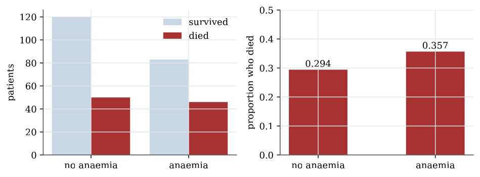
Anaemia and death
Worked example from Descriptive statistics
Question. Did patients with anaemia die more often?
Solution.
table(heart$anaemia, heart$death, dnn = c("anaemia", "death"))
proportions(table(heart$anaemia, heart$death), margin = 1)| Survived | Died | Proportion died | |
|---|---|---|---|
| No anaemia | 120 | 50 | 0.294 |
| Anaemia | 83 | 46 | 0.357 |
Row proportions, margin = 1, compare the death rate within each anaemia group: 29.4% without anaemia and 35.7% with it. The difference is six percentage points. Whether that is more than chance would produce with groups this size is a chi-squared test of independence, and it is not: the p-value is 0.25. High blood pressure gives 29.4% against 37.1%, with p-value 0.17, while for diabetes, sex and smoking the rates in the two groups differ by less than two percentage points.
A two-by-two table is a two-proportion test
Question page: A two-by-two table is a two-proportion test
Of 70 viewers of one channel, 40 are left-wing; of 100 viewers of another, 50 are. Compute the Pearson statistic for independence of channel and allegiance, and check that it equals the square of the pooled two-proportion z statistic, 0.918.
The table and its fitted counts R_iC_j/170 are
| Left | Not left | Total | |
|---|---|---|---|
| Channel 1 | 40 (37.06) | 30 (32.94) | 70 |
| Channel 2 | 50 (52.94) | 50 (47.06) | 100 |
| Total | 90 | 80 | 170 |
Every cell differs from its fitted count by 2.94 in absolute value, so
T=2.94^2\Bigl(\frac1{37.06}+\frac1{32.94}+\frac1{52.94}+\frac1{47.06}\Bigr)=0.843.
The pooled two-proportion statistic is z=0.918, and 0.918^2=0.843. The two statistics agree, and \chi^2_1 is the law of the square of a standard normal. The chi-squared p-value, 0.36, is the two-sided z test’s; the one-sided z test halves it.
Counting degrees of freedom
Question page: Counting degrees of freedom
Give the degrees of freedom of the Pearson statistic in each case. (a) A 4\times5 contingency table tested for independence. (b) Counts in 8 classes compared with a binomial distribution \operatorname{Bin}(7,p), with p estimated. (c) Counts in 10 classes compared with a normal distribution whose mean and variance are both estimated. (d) The same, with the mean and variance known.
(4-1)(5-1)=12.
8-1-1=6: eight classes, one estimated parameter.
10-1-2=7.
10-1=9: nothing is estimated.
Used in
- Taught in Chi-squared tests, where the derivation and examples are.
- Also used in Chi-squared examples
- All 4 questions on Chi-squared tests
See also
Pearson statistic · Pearson chi-squared approximation · Pearson test with estimated parameters