Question 19. Poisson regression for fish species
2024 examination, Question 3 (20 marks).
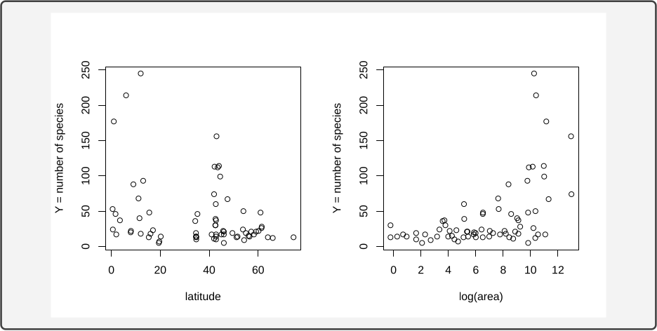
Barbour and Brown recorded the number Y_i of fish species in n=70 lakes, together with latitude and area. The scatterplots show the observed counts against the two covariates.
Consider
Y_i\mid X_i\stackrel{\mathrm{ind}}{\sim}\operatorname{Poisson}(\mu_i=\exp(X_i^{\top}\beta)), \qquad X_i^{\top}\beta=\beta_0+\beta_1\,\mathrm{latitude}_i+\beta_2\log(\mathrm{area}_i).
(a) [1 mark] Briefly argue why \log(\mathrm{area}_i) is preferable to \mathrm{area}_i in the linear predictor.
(b) [2 marks] Show that the log-likelihood is
\ell(\beta\mid X,Y)=\sum_{i=1}^{n}\bigl\{Y_i(X_i^{\top}\beta)-\exp(X_i^{\top}\beta)\bigr\}+\text{constant}.
(c) [2 marks] Derive the score and show that
S(\beta)=\sum_{i=1}^{n}\frac{Y_i-\mu_i(X_i^{\top}\beta)}{\operatorname{Var}(Y_i\mid X_i)}\,\mu_i'(X_i^{\top}\beta)\,X_i.
(d) [1 mark] Show that S(\beta) is unbiased.
(e) [2 marks] Verify \operatorname{Var}(S(\beta))=-\mathbb{E}[\partial S(\beta)/\partial\beta].
The first statistician fits the linear Poisson model:
fit1 = glm(species ~ latitude + log(area), family=poisson)

Coefficients:
             Estimate Std. Error z value Pr(>|z|)
(Intercept)  2.5949644  0.0668158   38.84   <2e-16 ***
latitude    -0.0149475  0.0008788  -17.01   <2e-16 ***
log(area)    0.2092975  0.0068808   30.42   <2e-16 ***

(Dispersion parameter for poisson family taken to be 1)
Null deviance:     2646.1 on 69 degrees of freedom
Residual deviance: 1249.9 on 67 degrees of freedom
AIC: 1616.4
(f) [5 marks] Interpret the intercept, the latitude and \log(\mathrm{area}) coefficients, the null deviance and the residual deviance.
The second statistician replaces the latitude slope with a smooth:
library(mgcv)
fit2 = gam(species ~ s(latitude) + log(area), family=poisson)

Parametric coefficients:
             Estimate Std. Error z value Pr(>|z|)
(Intercept)  2.064885   0.065793   31.39   <2e-16 ***
log(area)    0.202381   0.007701   26.28   <2e-16 ***

Approximate significance of smooth terms:
             edf Ref.df Chi.sq p-value
s(latitude) 8.881  8.996  463.2  <2e-16 ***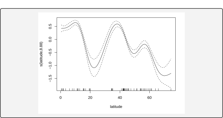
(g) [1 mark] Interpret the edf value 8.881.
(h) [2 marks] Comparing the two fits, is a linear function of latitude enough after accounting for lake area?
(i) [4 marks] Summarise the main findings in one short paragraph.
Definitions. Y_i is the species count in lake i, and X_i=(1,\mathrm{latitude}_i,\log\mathrm{area}_i)^\top is its fixed covariate vector. The model assumes independent Y_i\sim\operatorname{Poisson}(\mu_i) with \mu_i=\exp(X_i^\top\beta). Thus \mathbb{E}(Y_i\mid X_i)=\operatorname{Var}(Y_i\mid X_i)=\mu_i, with dispersion fixed at one. The score is the gradient of the log-likelihood, and Fisher information measures its expected curvature, or equivalently its covariance under the model.
(a) \log(\mathrm{area}) transforms a covariate; the log link transforms the response mean. These are separate choices. Logging area compresses its range and represents multiplicative area comparisons by additive differences: one unit of \log(\mathrm{area}) multiplies area by e. With a log link and a log-area predictor,
\mu_i=e^{\beta_0+\beta_1\mathrm{latitude}_i}\, \mathrm{area}_i^{\beta_2}.
This is a power-law area effect, whereas using raw area in the same log-link GLM gives an exponential area effect. The observed plot and scientific context should guide that choice; logging a covariate does not by itself establish model adequacy. Neither choice requires taking \log Y_i, so zero species counts pose no transformation problem for the response.
(b) The Poisson log-likelihood contribution is Y_i\log\mu_i-\mu_i-\log(Y_i!). The factorial term does not depend on \beta. With the log link, \log\mu_i=X_i^{\top}\beta and \mu_i=\exp(X_i^{\top}\beta), so
\ell(\beta\mid X,Y) = \sum_{i=1}^{n}\bigl\{Y_i(X_i^{\top}\beta)-\exp(X_i^{\top}\beta)\bigr\} +\text{constant}.
(c) Differentiate (b). Since \partial\mu_i/\partial\beta=\mu_i X_i,
S(\beta) = \sum_{i=1}^{n}(Y_i-\mu_i)X_i.
For every GLM the score is the same residual, reweighted by the variance and by the slope of the mean:
S(\beta) = \sum_{i=1}^{n} \frac{Y_i-\mu_i}{\operatorname{Var}(Y_i\mid X_i)} \,\mu_i'(X_i^{\top}\beta)\,X_i.
Here \operatorname{Var}(Y_i\mid X_i)=\mu_i. Under the log link, \mu_i'=\mu_i, so the weight equals 1 and the general score reduces to the sum above. Setting S(\beta)=0 is still nonlinear in \beta, because \mu_i=\exp(X_i^{\top}\beta). The fit is Fisher scoring of that equation, not a closed form.
(d) At the \beta in the model, \mathbb{E}(Y_i\mid X_i)=\mu_i. Each summand then has conditional mean zero, and \mathbb{E}[S(\beta)]=0.
Explicitly, with the design held fixed,
\mathbb{E}\{S(\beta)\mid X\} =\sum_iX_i\{\mathbb{E}(Y_i\mid X)-\mu_i\}=0.
This identity concerns repeated samples at the true parameter. The fitted score S(\hat\beta)=0 instead follows from maximising the observed likelihood; the two zeroes arise for different reasons.
(e) From the reduced score and \partial\mu_i/\partial\beta^{\top}=\mu_i X_i^{\top},
\frac{\partial S(\beta)}{\partial\beta} = -\sum_{i=1}^{n}\mu_i X_iX_i^{\top}.
The right-hand side does not depend on Y, so
-\mathbb{E}\!\left[\frac{\partial S(\beta)}{\partial\beta}\right] = \sum_{i=1}^{n}\mu_i X_iX_i^{\top}.
Calculate the score covariance separately. Conditional independence removes cross-covariances, and the Poisson variance is \operatorname{Var}(Y_i\mid X)=\mu_i, so
\operatorname{Var}\{S(\beta)\mid X\} =\sum_{i=1}^{n}\operatorname{Var}(Y_i\mid X)X_iX_i^{\top} =\sum_{i=1}^{n}\mu_iX_iX_i^{\top}.
This matches the negative expected Hessian above. The common matrix is the Fisher information. For the Poisson log link the observed and expected information agree; overdispersion or dependence would change the score covariance even if the mean formula remained correct.
(f) The intercept 2.595 is the log mean at latitude 0 (the equator) and \log(\mathrm{area})=0 (unit area), so the fitted mean there is \exp(2.595)\approx 13.4 species. This is the model’s reference lake, not a general mean for the sampled lakes.
The latitude coefficient -0.01495 is a multiplicative effect at fixed log area. One extra degree away from the equator multiplies the mean count by \exp(-0.01495)\approx 0.985. A degree is a small unit: ten degrees multiply the mean by \exp(-0.1495)\approx 0.861. Those are the same fit. The coefficient looks small because the unit is one degree.
The coefficient 0.2093 is the effect of one unit of \log(\mathrm{area}) at fixed latitude. Multiplying area by e multiplies the mean count by \exp(0.2093)\approx 1.233.
For any positive multiplier c, the fitted mean ratio is c^{0.2093}. Doubling area therefore multiplies the fitted mean by about 1.16, rather than by 1.23. The coefficient is an elasticity: a small 1\% increase in area corresponds to approximately a 0.2093\% increase in the expected count, holding latitude fixed.
The null deviance 2646.1 on 69 degrees of freedom is the deviance of the intercept-only model, one mean for every lake. The deviance is twice the drop in log-likelihood from the saturated fit to the model under discussion,
D(Y;\hat\mu)=2\bigl\{\ell(Y;Y)-\ell(\hat\mu;Y)\bigr\},
with Poisson dispersion fixed at 1. The degrees of freedom are n-1=69.
The residual deviance 1249.9 on 67 degrees of freedom is the deviance of the fitted three-parameter model, n-3=67. For the Poisson,
D = 2\sum_{i=1}^{n} \left\{ Y_i\log\frac{Y_i}{\hat\mu_i}-(Y_i-\hat\mu_i) \right\}.
The value is about 19 times its degrees of freedom, so the Poisson model fits poorly relative to its stated mean–variance assumptions. This can reflect overdispersion, a misspecified mean function, influential lakes or dependence; the deviance alone does not identify which. A quasi-Poisson fit with \operatorname{Var}(Y_i\mid X_i)=\phi\mu_i would retain these fitted coefficients while adjusting their standard errors, but it would not repair a wrong mean function.
The saturated fit has one fitted mean per observation, \hat\mu_i=Y_i, and hence no residual degrees of freedom. The null and residual degrees of freedom reveal n=70 and three fitted regression coefficients. In the deviance formula use 0\log(0/\hat\mu_i)=0 when Y_i=0. Comparing deviance to degrees of freedom is a diagnostic, not a proof that one particular assumption failed; sparse counts can also make a nominal chi-squared approximation inaccurate.
(g) The value 8.881 is the effective degrees of freedom of the fitted latitude smooth. It measures the smooth’s effective flexibility after penalisation, roughly comparable to a high-order polynomial fit; the fitted function is not literally a polynomial of degree 8.881. A value near 1 would indicate an approximately straight effect on the log-mean scale. Here the fitted effect is substantially more flexible.
The GAM keeps the Poisson response distribution and log link but replaces \beta_1\mathrm{latitude} by a fitted function g(\mathrm{latitude}). A smooth can be represented by basis functions with a penalty discouraging excessive wiggliness. The edf describes the flexibility remaining after that penalty, rather than the number of knots or an ordinary polynomial degree. The plotted ordinate is the smooth’s contribution to the log mean; obtaining a predicted count also requires the intercept and log-area contribution.
(h) The plotted effect of latitude rises and falls several times, so a single straight line on the log-mean scale misses its shape. The edf of 8.881 is also far above the near-linear value of 1. The printed \chi^2 test concerns whether the smooth is absent, not specifically whether it departs from a line. A direct formal comparison of linear and smooth latitude fits would address that narrower hypothesis. The log-area coefficient is similar in the two fits, 0.209 and 0.202.
(i) At a fixed latitude, multiplying lake area by e multiplies the fitted mean species count by about 1.23; the log-area coefficient stays close to 0.20 in the GAM. The smooth suggests high diversity near the equator, a dip around 20–25 degrees away, a rise around 30–40 degrees, and lower diversity towards the poles. A single latitude slope misses this pattern. The linear Poisson fit reduces deviance from 2646.1 to 1249.9, but the residual deviance remains far above 67 degrees of freedom. Check the mean function, the Poisson variance assumption and influential lakes before relying on its printed standard errors and z tests.