Question 22. Orthodontic growth curves
2025 examination, Question 4 (20 marks).
Distance from pituitary to pterygomaxillary fissure was measured every two years from age 8 to 14 on 27 subjects. The individual trajectories are shown below.
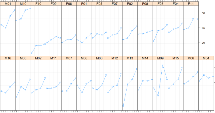
The random-slope fit fit1 = lmer(distance ~ age + Sex + (age|Subject)) has the following summary output:
Random effects:
 Groups   Name        Variance Std.Dev. Corr
 Subject  (Intercept)  7.82249   2.7969
          age          0.05126   0.2264 -0.77
 Residual              1.71621   1.3100
Number of obs: 108, groups: Subject, 27

Fixed effects:
             Estimate Std. Error t value
(Intercept)  17.63518    0.88623  19.899
age           0.66019    0.07125   9.265
SexFemale    -2.14544    0.75746  -2.832
(a) [6 marks] Write the statistical model for the random-slope command.
(b) [6 marks] Interpret the three fixed-effect estimates and the three standard deviations above.
ranef(fit1)$Subject
       (Intercept)         age
M16     -0.96698456 -0.06544230
F10     -2.31273350 -0.13319695
(c) [4 marks] Interpret the two pairs of predicted random effects.
fit2 = lmer(distance ~ age + Sex + (1|Subject))
anova(fit2, fit1)

      npar    AIC    BIC  logLik deviance  Chisq Df Pr(>Chisq)
fit2     5 444.86 458.27 -217.43   434.86
fit1     7 446.84 465.61 -216.42   432.84 2.0213  2     0.364
(d) [2 marks] Write the model for distance ~ age + Sex + (1|Subject).
(e) [2 marks] Is the random-intercept model an acceptable simplification?
Definitions. Y_{ji} is the orthodontic distance in millimetres for child j at occasion i, and age is in years. Set F_j=1 for female and 0 for male. A random-intercept-and-slope model has a child-specific pair (\alpha_{0j},\alpha_{1j}) with mean zero and covariance \Sigma_A. The residual error represents occasion-specific variation after the child’s own line has been accounted for. All variance components have units determined by the quantity they vary.
(a) Index the subject by j and the occasion by i. Male is the reference level of sex. The command (age|Subject) is a random intercept and a random slope on age, with a covariance between them:
\begin{aligned} Y_{ji} &= \beta_0+\beta_1\,\mathrm{age}_{ji}+\beta_2\,\mathrm{Female}_j + \alpha_{0j}+\alpha_{1j}\,\mathrm{age}_{ji} +\varepsilon_{ji},\\[4pt] \begin{pmatrix}\alpha_{0j}\\ \alpha_{1j}\end{pmatrix} &\sim \operatorname{N}(0,\Sigma_A), \qquad \varepsilon_{ji}\sim \operatorname{N}(0,\sigma^2), \end{aligned}
independently across subjects, with the errors independent of the random effects. From the fit,
\Sigma_A = \begin{pmatrix} 7.822 & -0.488\\ -0.488 & 0.0513 \end{pmatrix}, \qquad \sigma=1.310,
where -0.488\approx-0.77\times2.797\times0.226. Fixed effects are unknown population constants; random effects are realised child-specific departures modelled as draws from a population distribution. A new sample of children would have new realised departures, while the model’s population parameters describe the same population. The fit estimates both the mean structure and its variance components, using restricted maximum likelihood for the displayed fit.
The correlation -0.77 says that a child with a higher intercept tends to have a flatter slope. The intercept in this parameterisation is the value at age 0.
For distinct occasions at ages s and t on the same child, the model implies
\operatorname{Cov}\{Y_j(s),Y_j(t)\} =\tau_0^2+(s+t)\tau_{01}+st\tau_1^2,
where \tau_0^2,\tau_1^2,\tau_{01} are the entries of \Sigma_A. At a single occasion the variance additionally includes \sigma^2. This follows by expanding \operatorname{Cov}(\alpha_{0j}+s\alpha_{1j},\alpha_{0j}+t\alpha_{1j}); independent residual errors contribute no covariance between distinct occasions. It explains why ordinary independent-error regression is not the stated model.
(b) These six numbers are statements about the population, not about the 27 children in the file.
The intercept 17.635 mm is the extrapolated male mean at age 0. The measured ages run from 8 to 14, so this is outside the observed age range and should not be presented as a typical observed distance. At age 12, for example, the fitted male population mean is 17.635+0.660(12)=25.555 mm, a comparison within the measured range.
The age coefficient 0.660 mm per year is the population mean change for one extra year of age, the same slope for both sexes. The female coefficient -2.145 mm is the female mean minus the male mean at the same age.
The intercept standard deviation 2.797 mm says that a typical child sits about 2.8 mm away from the population intercept. That intercept is the age-0 value. The age standard deviation 0.226 mm per year says that a typical slope sits about 0.23 mm per year away from 0.660. The residual standard deviation 1.310 mm is the within-child scatter about that child’s own line.
The first two standard deviations describe between-child heterogeneity in line parameters; the last describes variation of measurements around a given child’s line. They are not standard errors of the fixed effects. Recentring age at 12 would make the intercept refer to a meaningful age and would change the random-intercept variance and intercept–slope correlation, while leaving fitted trajectories unchanged. Consequently the negative correlation must be interpreted with its age-0 reference in mind.
(c) The pairs (-0.967,-0.065) and (-2.313,-0.133) are predicted random effects for the sampled children. With the variances estimated, they are empirical best linear unbiased predictors. These values are departures from the appropriate population intercept and slope, so they must be added to the fixed part before a child’s fitted line is obtained.
For M16 the predicted line lies 0.967 mm below the male population intercept and 0.065 mm per year below the population slope:
(17.635-0.967)+(0.660-0.065)\,\mathrm{age} = 16.67+0.595\,\mathrm{age}.
For F10 the sex contrast is already in the fixed part. The predicted line lies a further 2.313 mm below the female intercept and 0.133 mm per year below the population slope:
(17.635-2.145-2.313)+(0.660-0.133)\,\mathrm{age} = 13.18+0.527\,\mathrm{age}.
These predictions pool each child’s measurements with the population model, shrinking poorly determined individual departures towards zero. They are not four additional fixed-effect coefficients. The fitted line predicts the child’s conditional mean; a future observed distance also has residual variation with standard deviation \sigma and uncertainty in the predicted line.
(d) Dropping the random slope leaves a common age slope and one random intercept:
Y_{ji} = \beta_0+\beta_1\,\mathrm{age}_{ji}+\beta_2\,\mathrm{Female}_j +\alpha_{0j}+\varepsilon_{ji},
with \alpha_{0j}\sim \operatorname{N}(0,\sigma_A^2) and \varepsilon_{ji}\sim \operatorname{N}(0,\sigma^2), independent across subjects. Two occasions on the same child then have covariance \sigma_A^2.
The corresponding within-child correlation is \sigma_A^2/(\sigma_A^2+\sigma^2) and is constant across pairs of distinct ages. Removing the random slope therefore imposes both a common age slope and a simpler covariance pattern. It still allows children to have persistently higher or lower distances through their random intercepts.
(e) Start from the larger model and delete. The likelihood-ratio statistic for the random slope and its covariance is 2.02 on 2 degrees of freedom, and the printed tail probability is 0.364. The random-intercept model has the smaller AIC, 444.86 against 446.84.
The null sets a variance to zero, a boundary of the parameter space, so the ordinary chi-squared reference used for the printed p-value is only approximate here. The large printed value and the lower AIC of the simpler model both support using the random-intercept model as an acceptable simplification for these data. This is not evidence that every subject has exactly the same age slope.
The larger model adds a slope variance and its covariance with the intercept, accounting for the two-parameter difference in the printed comparison. Both models must be fitted to the same observations and use a comparable likelihood criterion. Here the fixed-effects structure is the same, which permits a REML comparison of their random-effects structures. If fixed effects were being changed, the models should instead be compared using maximum likelihood. The statistical conclusion is that the extra random-slope structure is not sufficiently supported by these data, rather than that individual growth rates are known to be identical.