Autoregression and moving averages
Section of Dependence along a series, part of Time series
Autoregression and moving averages
| Type | Section |
| Taught in | Dependence along a series |
| Part | Time series |
| Questions using it | 6 |
An autoregression of order 1 writes X_t=\beta X_{t-1}+\varepsilon_t, with the innovations \varepsilon_t independent of each other. A random walk is the case \beta=1, and it wanders off. A spring temperature might have \beta a little above 1, a drift toward summer, plus a daily innovation. A winter temperature might have \beta a little below 1. The best guess of today’s temperature, before the day is observed, is often yesterday’s. A Markov chain is the same skeleton: the next state depends on the current state and a draw.
A moving average of order 1 depends on the previous innovation rather than the previous level: X_t=\alpha\varepsilon_{t-1}+\varepsilon_t. Stock that did not sell yesterday, discounted and sold today, plus a new surplus, is that equation. So is a weather forecast whose credibility today depends on how wrong it was yesterday, with \alpha the weight on yesterday’s error.
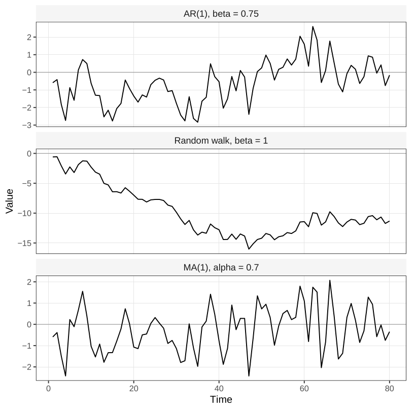
A series we record is a finite piece of a process that could have been running for a long time, and often in continuous time. A city’s midday temperature on 365 days is a sample from a continuous temperature path, taken at one hour of each day. The whole process can be studied first, and finite collections of times examined afterwards, which is the probabilist’s direction. Or a model can be written for the finite collection observed, which is the statistical direction. If every finite subcollection is multivariate normal, the continuous-time process is a Gaussian process, and the converse holds too. That equivalence is special to the normal. It is also why a Gaussian-process prior has become a fashionable smoother: one draw of the process is a curve, and a penalty on how irregular the draw is plays the role of \lambda in the smoothing chapters.
Used in
- Taught in Dependence along a series
- Also used in Graphical models · Forecasting
- Questions that use it (6) — A three-variable chain (answer) · C44 · C46 · C47 (answer) · C48 · C50 (answer)
- All 7 questions on Dependence along a series
See also
Autocorrelation function · Partial autocorrelation · ARCH and GARCH models · ARIMA model · Unit root · White noise · Wold decomposition · Stationarity of a time series