Monte Carlo method
Topic of Markov chains, Gibbs sampling, and Metropolis–Hastings, part of Bayesian statistics · Also in Hierarchical Bayes
Monte Carlo method
| Type | Topic |
| Taught in | Markov chains, Gibbs sampling, and Metropolis–Hastings · Hierarchical Bayes |
| Part | Bayesian statistics |
| Questions using it | 8 |
Approximating an expectation by an average over simulated draws, \mathbb{E}g(\theta)\approx\frac1M\sum_{m=1}^Mg(\theta^{(m)}). For independent draws the Monte Carlo error shrinks like 1/\sqrt M; correlated MCMC draws carry less information per draw.
In Markov chains, Gibbs sampling, and Metropolis–Hastings
MCMC is not intrinsically Bayesian. It is a general method for sampling difficult distributions, and it has deep roots in statistical physics as well as major uses in machine learning. Bayesian posterior calculation is one particularly natural application. The practical migration came at about 1990: methods long used in statistical physics, particularly condensed-matter problems involving large interacting systems, were taken up for posterior calculations that had previously been restricted largely to analytically convenient models. The recipe is to construct a chain whose equilibrium distribution is the posterior, then use its dependent output as a Monte Carlo sample.
In Hierarchical Bayes
From Hierarchical Bayes
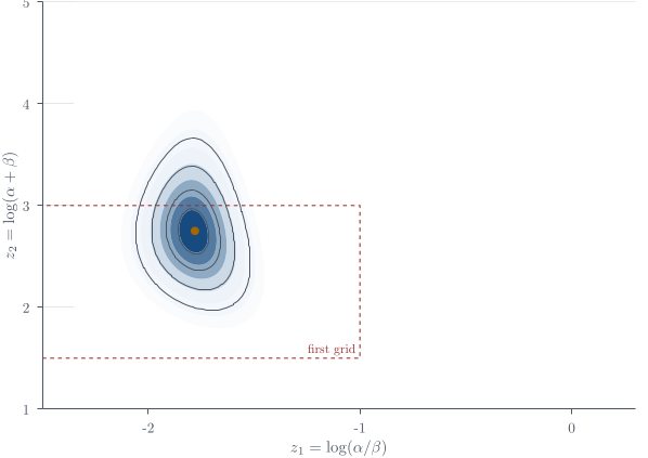
The calculation begins with a rectangular grid over (z_1,z_2), evaluates the unnormalised transformed hyperposterior at each cell, and expands the grid if substantial mass lies against an edge. The first trial used approximately
z_1\in[-2.5,-1], \qquad z_2\in[1.5,3],
and clipped part of the high-density region. An illustrative adjusted range was approximately
z_1\in[-2.35,0.3], \qquad z_2\in[1,5].
The grid method is deliberately visible. Modern MCMC software can hide much of this computation, but it still faces the same posterior geometry. A grid forces us to inspect the transformed scale, the Jacobian, the region carrying mass, and whether density is being clipped at a boundary. In two dimensions that transparency is often worth more than a more sophisticated black box.
Definition 1 (Grid Monte Carlo approximation) Let w_{ab} be the unnormalised hyperposterior value at grid cell (a,b), including the Jacobian \alpha\beta. The discrete approximation is
\widehat p_{ab}=\frac{w_{ab}}{\sum_{r,s}w_{rs}}.
Sampling from the approximate full posterior proceeds as follows.
Flatten the grid weights into a one-dimensional list, form cumulative probabilities, draw U\sim\operatorname{Uniform}(0,1), and select the first cell whose cumulative probability exceeds U. Equivalently, draw a grid cell (Z_1,Z_2) with probabilities \widehat p_{ab}. Optionally add independent uniform jitter within the selected cell.
Transform (Z_1,Z_2) to (\alpha,\beta) using Equation (10) in Hierarchical Bayes.
For each study, draw independently
\theta_j\sim\operatorname{Beta}(y_j+\alpha,n_j-y_j+\beta)
using Equation (7) in Hierarchical Bayes.
- Repeat to obtain (\alpha^{(l)},\beta^{(l)},{\boldsymbol{\theta}}^{(l)}), l=1,\ldots,L.
These grid-cell draws are independent; this is Monte Carlo from a piecewise-constant approximation, not Markov-chain Monte Carlo. A 100\times100 grid has 10^4 cells and remains practical because only two hyperparameters are integrated numerically. A comparable grid over all J+2 unknowns would be impossible.
Here is the corresponding calculation. The vectors y and n_trials contain the tumour counts y_j and sample sizes n_j for the 71 studies. The logarithmic calculation is important: subtracting the largest log weight before exponentiating prevents numerical underflow without changing the normalised probabilities.
z <- expand.grid(
  z1 = seq(-2.35, 0.30, length.out = 100),
  z2 = seq( 1.00, 5.00, length.out = 100)
)
total <- exp(z$z2)
mean_rate <- plogis(z$z1)
z$alpha <- total * mean_rate
z$beta  <- total * (1 - mean_rate)

log_w <- vapply(seq_len(nrow(z)), function(k) {
  a <- z$alpha[k]
  b <- z$beta[k]
  -2.5 * log(a + b) +
    sum(lbeta(y + a, n_trials - y + b) - lbeta(a, b)) +
    log(a) + log(b)              # Jacobian alpha * beta
}, numeric(1))

prob <- exp(log_w - max(log_w))
prob <- prob / sum(prob)

set.seed(3500)
M <- 1000L
cell <- sample.int(nrow(z), M, replace = TRUE, prob = prob)
alpha <- z$alpha[cell]
beta  <- z$beta[cell]
theta <- vapply(seq_along(y), function(j) {
  rbeta(M, y[j] + alpha, n_trials[j] - y[j] + beta)
}, numeric(M))
Each row of theta is one draw of all 71 study rates. Summarising a column marginalises (\alpha,\beta) automatically because the corresponding hyperparameter draws are simply not retained in that summary. Before using the result, plot the grid weights and check that appreciable mass does not meet an edge; a grid whose boundary cuts through the density fails precisely that check.
For a posterior expectation,
\mathbb{E}(\alpha\mid{\boldsymbol{y}}) \approx\frac1L\sum_{l=1}^L\alpha^{(l)}.
If the inferential target is only {\boldsymbol{\theta}}, marginalise the hyperparameters by ignoring their sampled coordinates and summarising {\boldsymbol{\theta}}^{(1)},\ldots,{\boldsymbol{\theta}}^{(L)}. This is Monte Carlo marginalisation, not a claim that hyperparameter uncertainty is absent.
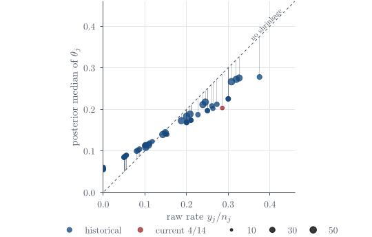
Study-specific posterior medians and 95\% intervals, ordered by the raw rates y_j/n_j, do not follow the 45-degree line: small and noisy studies move toward the population centre. This is shrinkage, also called borrowing strength. No observation is literally passed from one study to another. All studies help estimate the shared population quantities, and those quantities then influence every study-specific posterior. The model does not force the rates to be equal; the amount of movement is learned from the between-study spread and each study’s sample size.
Compared with plugging in one estimate of (\alpha,\beta), full Bayes usually widens the marginal intervals for \theta_j because it adds the variance due to hyperparameter uncertainty. Omitting that variance component makes the intervals over-precise.
The hierarchy shares information without forcing all studies to have the same rate. Full Bayes propagates uncertainty in the population of rates into every study-specific posterior. The grid sampler works because only two hyperparameters require numerical integration; in higher dimensions one would normally return to Gibbs or Metropolis–Hastings.
Used in
- Taught in Markov chains, Gibbs sampling, and Metropolis–Hastings · Hierarchical Bayes
- Also used in Discrete-time Markov chains · Bayesian foundations · The Beta–Binomial model · Hierarchical Bayes
- Questions that use it (8) — Metropolis–Hastings for the logit-normal posterior (answer) · Restaurant ordering methods (answer) · Q19 (answer) · Q25 (answer) · Question 3 (answer) · Question 9 (answer) · C11 · C15 (answer)
- All 31 questions on Markov chains, Gibbs sampling, and Metropolis–Hastings
See also
Expectation · Posterior summaries from draws · Markov chain · Effective sample size · Grid Monte Carlo approximation · R’s distribution interface · Thinning a Markov chain · Stationarity and detailed balance