Ordinal responses

Section of Categorical responses, part of Generalised linear models

Ordinal responses

Type	Section
Taught in	Categorical responses
Part	Generalised linear models
Questions using it	2

Food scores, pain scores, and agreement scales have cutpoints that are partly conventional. If we collapse “strongly agree” into “agree”, the form of the model should survive. The estimates will change, because information was thrown away. The equation should be the same kind of equation. That requirement is what forces cumulative probabilities rather than a separate model for each p_k.

Three categories are enough to see it. In the pneumonia experiment, animals were exposed to a bacterium for a logged time x=\log(\text{exposure in seconds}), and the response was 1 none, 2 mild, 3 severe. Sample size falls as the dose rises, which is the ethical constraint you would hope for. The rows, with x=\log t, are

seconds	x	none	mild	severe
5.8	1.76	98	0	0
15.0	2.71	51	2	1
21.5	3.07	34	6	3
27.5	3.31	35	5	8
33.5	3.51	32	10	9
39.5	3.68	23	7	8
46.0	3.83	12	6	10
51.5	3.94	4	2	5

Suppose the only question is whether any pneumonia occurred. Mild and severe collapse into one category, and the problem is binary: \mathrm{P}(Y\ge 2)=\frac{\exp(\beta_{0,\mathrm{ms}}+\beta_{1,\mathrm{ms}} x)}{1+\exp(\beta_{0,\mathrm{ms}}+\beta_{1,\mathrm{ms}} x)}. Suppose instead that mild disease is treatable and only severe disease is the event. None and mild collapse, and again the problem is binary, with its own intercept and slope, for \mathrm{P}(Y\ge 3). The only model for three ordered categories that collapses to a logistic regression on every neighbouring split is a logistic regression for each upper tail: \begin{align*} \mathrm{P}(Y\ge 3)&=\frac{\exp(\beta_{03}+\beta_{13}x)}{1+\exp(\beta_{03}+\beta_{13}x)},\\ \mathrm{P}(Y\ge 2)&=\frac{\exp(\beta_{02}+\beta_{12}x)}{1+\exp(\beta_{02}+\beta_{12}x)},\\ \mathrm{P}(Y\ge 1)&=1. \end{align*} That is an interaction: every cutpoint has its own slope. It is as hard to read as a set of non-parallel lines. The model we fit forces the slopes to be common and lets only the intercepts differ.

Definition 1 A proportional-odds model for ordered categories 1,\ldots,K and covariates {\boldsymbol{x}} is \mathrm{logit}\,\mathrm{P}(Y\ge k\mid {\boldsymbol{x}})=\beta_{0k}+{\boldsymbol{x}}^\top\boldsymbol{\beta}, \qquad k=2,\ldots,K, with \beta_{02}\ge\beta_{03}\ge\cdots\ge\beta_{0K}. A unit increase in a covariate multiplies the odds of being in category k or higher by e^{\beta_j}, and that factor does not depend on k.

Article: Proportional-odds model →

The intercepts have to decrease as k increases, because \mathrm{P}(Y\ge 2)\ge\mathrm{P}(Y\ge 3)\ge\cdots. For a university grade, one extra hour of study multiplies the odds of a 4 or better, a 5 or better, and a 7, by the same factor. If those factors differed, you would have a non-proportional odds model, which is the interaction above, and we would not lead with it.

The response at each x is a vector of counts, so the fit is a vector GLM. In the VGAM package:¹

need <- function(pkg) {
  if (!requireNamespace(pkg, quietly = TRUE)) {
    install.packages(pkg, repos = "https://cloud.r-project.org")
  }
  suppressPackageStartupMessages(library(pkg, character.only = TRUE))
}
need("VGAM")
data(pneumo, package = "VGAM")
pneumo$none <- pneumo$normal
pneumo$x <- log(pneumo$exposure.time)
summary(vglm(cbind(none, mild, severe) ~ x, family = propodds, data = pneumo))

              Estimate Std. Error z value
(Intercept):1  -9.6761     1.3241   -7.31
(Intercept):2 -10.5817     1.3454   -7.86
x               2.5968     0.3811    6.81

The first linear predictor is \mathrm{logit}\,\mathrm{P}(Y\ge 2). The second is \mathrm{logit}\,\mathrm{P}(Y\ge 3). So \begin{align*} \widehat{\mathrm{P}}(Y\ge 2) &=\frac{\exp(-9.6761+2.5968\,x)}{1+\exp(-9.6761+2.5968\,x)},\\ \widehat{\mathrm{P}}(Y\ge 3) &=\frac{\exp(-10.5817+2.5968\,x)}{1+\exp(-10.5817+2.5968\,x)}. \end{align*}

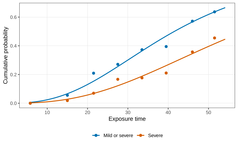
Figure 1: Fitted cumulative probabilities against exposure time. The severe curve stays below the curve for mild or severe, and the two curves share a slope on the logit scale. Points are the proportions in the table.

At x=0, which is one second of exposure if x is a natural log of seconds, the odds of severe pneumonia are e^{-10.58}, of order 10^{-5}. The odds of mild or severe are e^{-9.68}, larger, as they must be, because that event contains the severe cases. Both are negligible, which is the right answer for an animal that was barely exposed.

A unit increase in x is a factor of e\approx 2.7 in exposure time, roughly a threefold increase. It multiplies the odds of crossing either cut by \exp(2.5968)=13.4. The z statistic on that slope is 6.81. Exposure time is strongly associated with worse pneumonia, and the multiplier is the same for “any pneumonia” and for “severe pneumonia”. That is the proportional-odds claim.

Replacing the logit by the complementary log-log gives a proportional-hazards model, \log\bigl(-\log(1-\gamma_k)\bigr)=\beta_{0k}+{\boldsymbol{x}}^\top\boldsymbol{\beta}, with the same parallel-slope constraint and the same ordering of intercepts. The coefficient is a log hazard, not a log odds ratio. We can say what an odds ratio is. A hazard is a definition we can write down and a quantity we cannot usually explain. The call that forces the cumulative, reversed, parallel, complementary-log-log model is

need <- function(pkg) {
  if (!requireNamespace(pkg, quietly = TRUE)) {
    install.packages(pkg, repos = "https://cloud.r-project.org")
  }
  suppressPackageStartupMessages(library(pkg, character.only = TRUE))
}
need("VGAM")
data(pneumo, package = "VGAM")
pneumo$none <- pneumo$normal
pneumo$x <- log(pneumo$exposure.time)
fit <- vglm(cbind(none, mild, severe) ~ x,
            family = cumulative(reverse = TRUE, parallel = TRUE, link = "cloglog"),
            data = pneumo)
summary(fit)
deviance(fit)
logLik(fit)

and it returns intercepts -8.60 and -9.35, with slope 2.21 (z=7.06). The residual deviance is 6.65 against 5.03 for the proportional-odds fit, and the log-likelihood is -25.90 against -25.09. The odds model fits this table a little better. The two models are not nested, so that comparison is not a likelihood-ratio test. It is the same kind of absolute comparison as an AIC when the parameter count matches, which here it does.

Used in

Taught in Categorical responses
Questions that use it (2) — C24 · C25
All 3 questions on Categorical responses

Footnotes

The package is Thomas Yee’s, at the University of Auckland. The vector form is there because a three-category count is not a single Bernoulli column.↩︎

Used in

See also

Footnotes