Two-factor analysis of variance

Section of Analysis of variance examples, part of Data analysis

Type	Section
Taught in	Analysis of variance examples
Part	Data analysis

Many experiments vary more than one factor. The model for two factors, with d_1 and d_2 levels and n_{ij} observations in cell (i,j), is

Y_{ijk}=\mu+\alpha_i+\beta_j+\gamma_{ij}+\varepsilon_{ijk}, \qquad \varepsilon_{ijk}\ \text{independent}\ \operatorname{N}(0,\sigma^2).

Here \mu is a baseline mean, \alpha_i and \beta_j are the main effects of the two factors, and \gamma_{ij} is their interaction. The parameters are not all identifiable as written; R fixes them by setting the effects of the first level of each factor to zero.

Definition 1 (Interaction) Two factors interact when the effect of one depends on the level of the other: the difference in mean response between two levels of the first factor is not the same at every level of the second. In the two-factor model, there is no interaction when every \gamma_{ij}=0.

Article: Interaction →

An interaction plot draws the cell means of one factor against its levels, one line per level of the other factor. Parallel lines mean no interaction. With interaction present, the main effects on their own are hard to interpret: “the effect of fertilizer” is not a single number if it depends on the region.

The two-factor ANOVA table splits the total sum of squares into a part for each factor, a part for the interaction, and the error:

Source	Df	F
Factor 1	d_1-1	\mathrm{MS}_1/\mathrm{MSE}
Factor 2	d_2-1	\mathrm{MS}_2/\mathrm{MSE}
Interaction	(d_1-1)(d_2-1)	\mathrm{MS}_{12}/\mathrm{MSE}
Error	n-d_1d_2
Total	n-1

Testing for interaction needs replication: with one observation per cell there are no error degrees of freedom left once the interaction is fitted, which is why the randomised block design assumes no interaction.

Example 1 (Wheat in four regions) Three fertilizers were each tried three times in each of four regions, giving 36 wheat yields.

yield <- c(9.18, 8.26, 8.57, 10.05, 8.92, 9.39, 11.23, 11.11, 9.72, 11.60, 9.83, 11.07,
           9.69, 8.25, 9.83, 9.80, 10.90, 10.75, 12.13, 12.01, 9.67, 12.09, 10.15, 12.04,
           7.87, 8.91, 7.78, 8.33, 8.18, 9.78, 9.38, 10.10, 10.90, 11.73, 8.86, 11.23)
fertilizer <- gl(3, 12, 36, labels = paste("Fertilizer", 1:3))
region <- gl(4, 3, 36, labels = paste("Region", 1:4))
anova(lm(yield ~ region * fertilizer))
#                   Df Sum Sq Mean Sq F value    Pr(>F)
# region             3 29.340  9.7801 11.2388 8.451e-05
# fertilizer         2  8.560  4.2798  4.9182   0.01622
# region:fertilizer  6  0.695  0.1159  0.1332   0.99067
# Residuals         24 20.885  0.8702

Question. Do region and fertilizer affect yield, and do they interact?

Solution. The interaction is negligible: F=0.13 with p-value 0.99, and the interaction plot shows nearly parallel lines. Dropping it gives the additive model, lm(yield ~ region + fertilizer), whose error mean square, 0.719 on 30 degrees of freedom, pools the interaction into the error. Both main effects are then clear: region with F=13.6 and p=9\times10^{-6}, fertilizer with F=5.95 and p=0.007. Mean yields rise from 8.70 in region 1 to 10.96 in region 4; fertilizer 2 gives the highest mean, 10.61, against 9.91 and 9.42 for the others.

Analysing one region alone throws information away. In region 1 by itself, anova(lm(yield ~ fertilizer, subset = region == "Region 1")) gives F=1.87 and p=0.23: with only 9 observations, the error variance is poorly estimated, and the fertilizer effect that the full analysis finds is not visible.

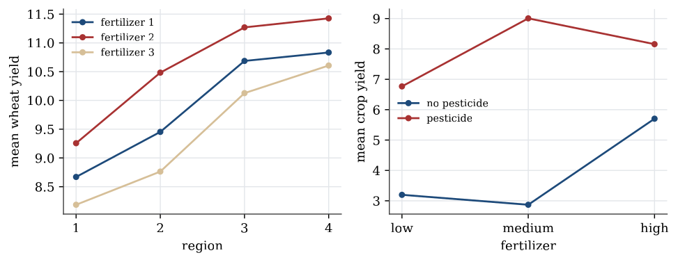
Figure 1: Interaction plots. Left: wheat yield means by region, one line per fertilizer; the lines are nearly parallel, so there is no interaction. Right: crop yield means by fertilizer level, one line per pesticide setting; the lines cross, a strong interaction.

Example 2 (Pesticide and fertilizer) A crop was grown with pesticide (no or yes) and fertilizer (low, medium or high), three plots per combination. The mean yields were

	Low	Medium	High
No pesticide	3.20	2.87	5.70
Pesticide	6.77	9.01	8.16

Question. What does a two-factor analysis show?

Solution. A two-sample t test of pesticide alone, ignoring fertilizer, gives t=-7.30 and p=1.8\times10^{-6}. The two-factor analysis with interaction shows why that single number is incomplete. The interaction is enormous, F=574 on (2,12) degrees of freedom: without pesticide the yield is best at high fertilizer, with pesticide it is best at medium. The effect of pesticide is 3.57 at low fertilizer, 6.14 at medium and 2.45 at high. Reporting one average “pesticide effect” would hide that the best fertilizer level depends on whether pesticide is used. With interaction this strong, the useful summary is the table of cell means.

Used in

Taught in Analysis of variance examples
All 2 questions on Analysis of variance examples

Used in

See also