Kyphosis data

Section of Smooth means, part of Smoothing

Kyphosis data

Type	Section
Taught in	Smooth means
Part	Smoothing

Eighty-one children were followed after spinal surgery to see whether kyphosis, a forward bend in the spine, was still present. Age is recorded in months, from infancy out to about 200 months. The ones and zeros rise through the middle ages and fall again. A logistic regression with age as a linear predictor can only ever increase, or only ever decrease. It cannot come back down. So keep the logistic mean, and let the inside be a smooth function centred at zero: \mathrm{P}(\text{kyphosis}\mid \text{age}) =\frac{\exp\{\beta_0+g(\text{age})\}}{1+\exp\{\beta_0+g(\text{age})\}}, where g is constrained to average zero so that \beta_0 is the log-odds at the centre of the age effect. In mgcv,

need <- function(pkg) {
  if (!requireNamespace(pkg, quietly = TRUE)) {
    install.packages(pkg, repos = "https://cloud.r-project.org")
  }
  suppressPackageStartupMessages(library(pkg, character.only = TRUE))
}
need("mgcv")
need("rpart")
data(kyphosis, package = "rpart")
kyphosis$Kyphosis <- as.numeric(kyphosis$Kyphosis == "present")
fit <- gam(Kyphosis ~ s(Age), family = binomial, data = kyphosis)
summary(fit)

s(Age) asks for the smooth. Knots and \lambda are chosen by cross-validation. The plotted smooth is labelled with equivalent degrees of freedom 2.22: more flexible than a quadratic, short of a cubic, and not itself a polynomial of degree 2.22. It is a piecewise cubic whose overall budget of wiggliness is 2.22. The intercept is -1.51 (z=-4.78), so at the centre of g the odds are e^{-1.51}. The smooth term has \mathrm{edf}=2.22,\qquad \chi^2=6.69,\qquad p=0.071. The equivalent degrees of freedom and the intercept -1.51 are what the code prints. The chi-squared statistic moves with the version of mgcv: one printout was 6.69 with p=0.071, and mgcv 1.8 reports about 6.36 with p=0.076. Either reading is the same decision.

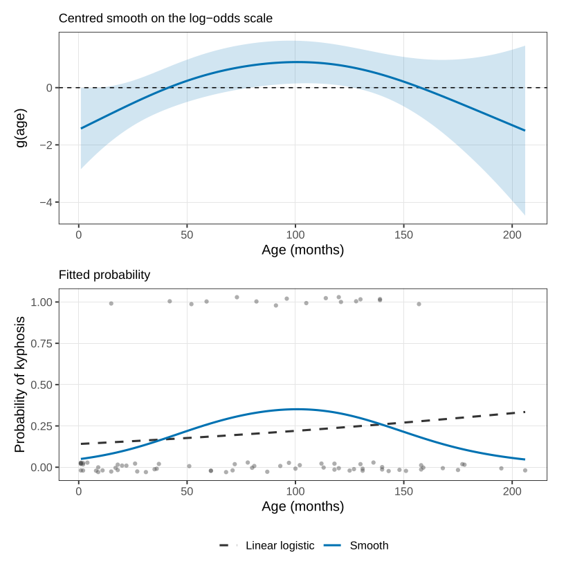
Figure 1: Top: the centred age smooth on the log-odds scale, with the confidence band drawn by mgcv. The dashed line at zero is “age does nothing”, and it just about stays inside the band. Bottom: the fitted probability. The dashed line is a logistic regression that is linear in age, and it cannot come back down.

In Figure a horizontal line at zero just about stays inside the band, and it just about fails to. We do not have a hard rule at 0.05. We keep age. The fitted probability, the expit of \beta_0+g, rises and then falls. That graph is the answer to “how does kyphosis depend on age?”. There is no unit-change sentence, and that is the price of not having specified the shape in advance.

The substantive reading we would offer, cautiously, is a mixture of biology and of who is sent to surgery. Very young children are operated on because the problem is serious, and they also recover more readily. Older adolescents are often milder cases, chosen for correction once the skeleton is more settled. The ages in the middle are the ones whose surgery was delayed and whose bones were no longer infant bones. You cannot randomise the age at which an elective operation happens. The curve is a description of this sample, not a pure age effect.

Number of vertebrae operated on, and where on the spine the operation started, are in the same data set. They are the next chapter. A smooth of age alone is the model this chapter stops on.

In the penalised criterion, what does the fitted g become as \lambda\to\infty, and what does it become as \lambda\to 0 if all the x_i are distinct?
The kyphosis smooth has equivalent degrees of freedom 2.22 and a p-value of about 0.07. Say what each of those numbers is measuring, and why a logistic regression that is linear in age cannot reproduce the shape in the plot.

Kyphosis data

Used in

See also