Lidar data
Section of Smooth means, part of Smoothing
Lidar data
| Type | Section |
| Taught in | Smooth means |
| Part | Smoothing |
Ruppert, Wand, and Carroll’s lidar data take Y to be the log ratio of received light to emitted light, and x the range in feet. A perfect return would sit at 0. Some points sit above 0 because the room is not dark: the sensor records the laser plus whatever else is shining. Out to roughly 500 or 550 feet the mean is flat. Past that threshold it drops, sharply, and the scatter widens as the mean falls. A laser gets weaker with distance and it gets noisier. The variance is a GLM problem, and we already know how to write \mathrm{Var}=\phi V(\mu). The mean is not a quadratic we would have written down before seeing the plot, and we would not want to have to name the threshold.
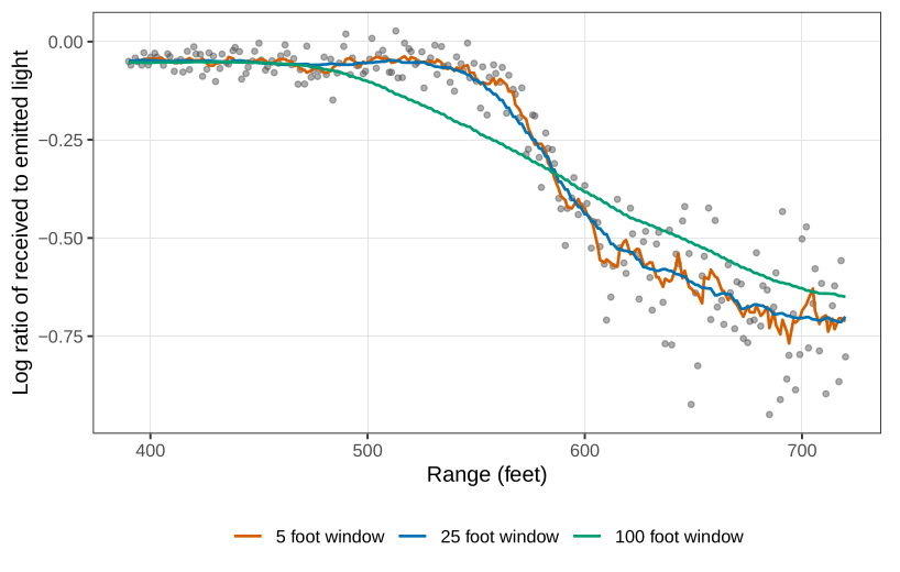
A moving window is the first smoother you are likely to have seen. In Figure, averaging within \pm 5 feet leaves a noisy curve. Within \pm 25 feet it is calmer but still jagged on the drop. Within \pm 100 feet it is smooth and it has smeared the drop. A single window width cannot be wide where the noise is large and narrow where the signal is sharp. The window also ignores the mean-variance relationship, so it oversmooths the precise part of the curve and undersmooths the noisy part. The penalty has to live on the likelihood scale, where a GLM already knows that a residual at a large mean is not the same as a residual at a small one.
Used in
- Taught in Smooth means
- All 5 questions on Smooth means
See also
Roughness penalty · Kyphosis data · Cubic smoothing spline · Spline · Knot