Roughness penalty
Section of Smooth means, part of Smoothing
Roughness penalty
| Type | Section |
| Taught in | Smooth means |
| Part | Smoothing |
Green and Silverman’s formulation is the clean one, even though we no longer compute it with a knot at every x. Keep the exponential family. Replace the linear predictor by an unknown smooth function g(x), and keep the canonical link, so the mean is -c'(g(x)). For the normal that is g(x) itself. For the Poisson it is \exp(g(x)), which stays positive whatever g does. For the Bernoulli it is the expit of g(x), which stays inside (0,1). For the gamma the canonical choice is 1/g(x), and that still requires g not to change sign. You may use a log link for the gamma instead. Nothing forces the canonical link once you have decided the mean is smooth rather than linear.
Maximise the log-likelihood and charge for curvature: \sum_{i=1}^n\bigl\{y_i g(x_i)-c(g(x_i))\bigr\} -\frac{\lambda}{2}\int \{g''(x)\}^2\,\mathrm{d}x. The first piece wants g to pass through the data. The integral of the squared second derivative is large when the curve turns often. A straight line has second derivative zero and pays nothing. A sine wave pays on every oscillation. \lambda is the exchange rate between fidelity and smoothness. The half is cosmetic: for the normal likelihood it cancels the usual factor of one half.
The maximiser, for any fixed \lambda, is a cubic spline with a knot at each distinct x_i. Inside each interval the function is a cubic. At each knot the function, the first derivative, and the second derivative agree from the left and the right. Your eye can see those three. It cannot see a jump in the third derivative, which is why a cubic, rather than a higher piecewise polynomial, is the one this penalty produces.
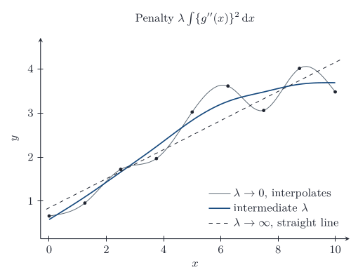
Putting a knot at every x_i is expensive, and \lambda itself changes meaning when you change the likelihood. In practice we use a smaller set of knots, ten equally spaced between the smallest and largest x being the usual default, or knots at the deciles if the x values pile up at one end. More knots are available when the sample is in the thousands. And we do not quote \lambda. Cross-validation hides a fraction of the sample, fits on the rest, and scores the hidden points, rotating which fraction is hidden. The software reports the smoothness as an equivalent degrees of freedom: the polynomial degree the curve is about as flexible as. As \lambda\to\infty that degrees of freedom falls to 1, a straight line, which is the ordinary GLM. As \lambda\to 0 the fit interpolates, and if no x values are tied it interpolates perfectly. Interpolation fits noise. It does not predict the next point.
Used in
- Taught in Smooth means
- Also used in Hierarchical clustering and kernel density estimation
- All 5 questions on Smooth means
See also
Cubic smoothing spline · Gaussian process · Effective degrees of freedom · Knot · Regularisation · Spline · Lidar data · Kyphosis data