Leaf-blotch data

Section of Underdispersion, positive responses, and quasi-likelihood, part of Generalised linear models

Leaf-blotch data

Type	Section
Taught in	Underdispersion, positive responses, and quasi-likelihood
Part	Generalised linear models

Wedderburn (1974) is the paper that introduced this. Ten barley varieties were grown at nine sites, one proportion per cell: the percentage of leaf area covered by blotch, Rhynchosporium secalis. The variety and site numbers in the table are labels, ordered roughly from less blotch to more. They are not numeric covariates. Treating “variety 2” as twice “variety 1” is the same mistake as averaging student ID numbers.

There is one observation per variety–site pair, so a full interaction cannot be fitted. The mean model is main effects only, on the logit of the proportion p_{ij}: \log\frac{p_{ij}}{1-p_{ij}}=\alpha_i+\beta_j, \qquad p_{ij}=\frac{\exp(\alpha_i+\beta_j)}{1+\exp(\alpha_i+\beta_j)}. A structured interaction would be allowed if a reason for that particular combination existed before looking at the table. It does not. The variance starts as quasi-binomial, \phi p(1-p). The proportions are averages of many leaves from the same plot, so the trials are not independent Bernoulli draws. Pseudo-replication makes \phi much smaller than 1.

need <- function(pkg) {
  if (!requireNamespace(pkg, quietly = TRUE)) {
    install.packages(pkg, repos = "https://cloud.r-project.org")
  }
  suppressPackageStartupMessages(library(pkg, character.only = TRUE))
}
need("faraway")
data(leafblotch, package = "faraway")
leafblotch$proportions <- leafblotch$blotch
summary(glm(proportions ~ factor(site) + factor(variety),
            data = leafblotch, family = quasibinomial))

The dispersion printed for this fit is \hat\phi=0.089. The intercept, -8.05, is the log-odds for variety 1 at site 1. Every other coefficient is a contrast with that baseline. After adjusting for site, varieties 2, 3, and 4 are not distinguishable from variety 1 at the 5% level (variety 2 even has t=0.21). Varieties 5 through 10 are worse. Variety 1 is the most resilient in this fit, with 2, 3, and 4 in the same neighbourhood.

The Pearson residual is (y_i-\hat\mu_i)/\sqrt{\hat\phi V(\hat\mu_i)}. Plotted against the linear predictor, these residuals are not a flat band. The quasi-binomial variance compresses the small fitted values too hard and does not compress the middle enough. Wedderburn’s replacement is V(\mu)=\mu^2(1-\mu)^2, still multiplied by a free \phi. Squaring p(1-p) shrinks the variance even more near 0 and 1, and it leaves relatively more variance in the middle, which is what the residual plot was asking for.

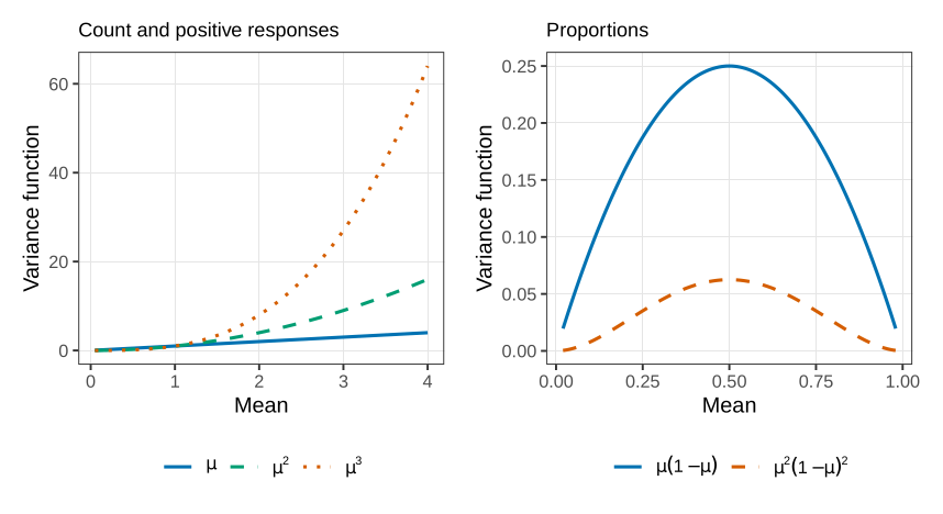
Figure 1: Variance as a function of the mean. On the left, mu, mu squared and mu cubed are the Poisson, gamma and inverse-Gaussian choices. On the right, the binomial variance and Wedderburn’s replacement: smaller in the tails, and relatively larger through the middle.

No exponential family has this variance function. It is a description. It is not a quasi-binomial. There is nothing to call it except a quasi-likelihood with this V.

It is not a built-in family. You supply V and its derivatives to glm. A proportion of exactly zero makes the quasi-deviance integral diverge, so the block below prints the variety contrasts and their standard errors, which do not need that integral.

need <- function(pkg) {
  if (!requireNamespace(pkg, quietly = TRUE)) {
    install.packages(pkg, repos = "https://cloud.r-project.org")
  }
  suppressPackageStartupMessages(library(pkg, character.only = TRUE))
}
need("faraway")
data(leafblotch, package = "faraway")
leafblotch$proportions <- leafblotch$blotch
wedderburn <- quasi(
  link = "logit",
  variance = list(
    varfun = function(mu) mu^2 * (1 - mu)^2,
    validmu = function(mu) all(mu > 0 & mu < 1),
    dev.resids = function(y, mu, wt) wt * (y - mu)^2 / (mu^2 * (1 - mu)^2),
    initialize = expression({
      n <- rep.int(1, nobs)
      mustart <- pmax(0.001, pmin(0.999, y))
    }),
    name = "mu^2(1-mu)^2"
  )
)
fit <- glm(proportions ~ factor(site) + factor(variety),
           data = leafblotch, family = wedderburn)
co <- coef(summary(fit))
round(co[grep("variety", rownames(co)), ], 3)

After that fit, the contrasts with variety 1, and a common standard error of 0.47 because the design is balanced, are

variety	1	2	3	4	5	6	7	8	9	10
contrast	0	-0.47	0.08	0.95	1.35	1.33	2.34	3.26	3.14	3.89

Variety 2 is now the most resilient, slightly ahead of variety 1. Varieties 1, 2, and 3 remain the resistant group: variety 4 is about two standard errors up, and from variety 5 the gap is clear. The ranking moved a little. The standard errors moved more, from about 0.6 down to 0.47, and the residual plot is closer to a constant-width scatter.

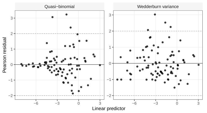
Figure 2: Pearson residuals against the linear predictor. On the left the quasi-binomial variance squeezes the small fitted values, at the left of the panel, onto the horizontal axis. On the right, Wedderburn’s variance gives those same points more room. Dashed lines are at plus or minus 2.

For a proportion that is actually continuous, a Pearson plot is a fair diagnostic. For a binary or count response the same plot bands, because the observation can only sit on a lattice, and that banding is not evidence against the mean. We will handle discrete residuals later.

Key idea

Once the mean is specified, any non-negative variance function V(\mu) gives a quasi-score that glm can solve. Whether that V is the variance of a named distribution is a separate question. A descriptive fit is allowed. It is not a generator of new data.

From the gamma interaction fit, recompute the second lot’s intercept and slope by adding the baseline coefficients to the lot.f2 coefficients, and write \mu_2 as a reciprocal.
Show \mathrm{E}(S_\mu)=0 and \mathrm{Var}(S_\mu)=1/(\phi V(\mu)) from the definition of S_\mu, using only \mathrm{E}(Y)=\mu and \mathrm{Var}(Y)=\phi V(\mu).
Explain why \hat{\boldsymbol{\beta}} in a quasi-model does not depend on \phi, and why \hat\phi in Equation (1) in Underdispersion, positive responses, and quasi-likelihood is computed only after \hat{\boldsymbol{\beta}}.
The leaf-blotch design has one observation per variety–site cell. Say why a product interaction site * variety is not available, and why that is different from refusing the interaction on scientific grounds.

Leaf-blotch data

Used in

See also