Positive continuous responses
Section of Underdispersion, positive responses, and quasi-likelihood, part of Generalised linear models
Positive continuous responses
| Type | Section |
| Taught in | Underdispersion, positive responses, and quasi-likelihood |
| Part | Generalised linear models |
A clotting time, or an insurance claim amount, is continuous and cannot be negative. Three links are in ordinary use: \begin{align*} \log\mu_i&={\boldsymbol{X}}_i^\top\boldsymbol{\beta}, & \mu_i&=\exp({\boldsymbol{X}}_i^\top\boldsymbol{\beta}),\\ \mu_i^{-1}&={\boldsymbol{X}}_i^\top\boldsymbol{\beta}, & \mu_i&=1/({\boldsymbol{X}}_i^\top\boldsymbol{\beta}),\\ \mu_i^{-2}&={\boldsymbol{X}}_i^\top\boldsymbol{\beta}, & \mu_i&=1/\sqrt{{\boldsymbol{X}}_i^\top\boldsymbol{\beta}}. \end{align*} The log link is the one with a direct reading, and it keeps \mu positive for every finite predictor. It is not the canonical link for the gamma or the inverse Gaussian, so R will not choose it unless you name it. The canonical link for the gamma is the inverse link. The canonical link for the inverse Gaussian is the inverse quadratic. Both of those are only positive when {\boldsymbol{X}}^\top\boldsymbol{\beta}>0. If the linear predictor changes sign, the inverse link produces a negative mean, and the square root in the inverse quadratic leaves the reals. It is sometimes said that the inverse quadratic “ensures” non-negativity because a complex mean is not a mean. That is a restriction on the domain of \boldsymbol{\beta}, not a guarantee for every coefficient vector. You still have to keep the linear predictor positive.
The two families are written by their mean and variance, so the shape-rate and shape-scale arguments do not have to be reconstructed: \begin{align*} Y_i\mid {\boldsymbol{X}}_i&\stackrel{\mathrm{ind}}{\sim}\mathrm{Gamma}\!\left(\mu_i=\mu({\boldsymbol{X}}_i^\top\boldsymbol{\beta}),\ \mathrm{Var}=\phi\mu_i^2\right),\\ Y_i\mid {\boldsymbol{X}}_i&\stackrel{\mathrm{ind}}{\sim}\mathrm{InverseGaussian}\!\left(\mu_i=\mu({\boldsymbol{X}}_i^\top\boldsymbol{\beta}),\ \mathrm{Var}=\phi\mu_i^3\right). \end{align*} The mean function \mu(\cdot) is whichever inverse link you chose. It is not tied to the family. The score for a gamma regression has the same shape as the Bernoulli and Poisson scores, (y-\mu)\mu'/\mathrm{Var}, and showing that is an exercise rather than a new idea. Intervals are again z intervals from the inverse Fisher information.
Clotting times, three ways
Main article: Clotting-time data
Return to the clotting data. Two lots of thromboplastin, log dose, clotting time in seconds. If a dose of zero is imagined to mean no clotting agent at all, an infinite mean time is the story the inverse link tells, and it is the default for family = Gamma. Fit an interaction, so each lot has its own intercept and its own slope:
need <- function(pkg) {
  if (!requireNamespace(pkg, quietly = TRUE)) {
    install.packages(pkg, repos = "https://cloud.r-project.org")
  }
  suppressPackageStartupMessages(library(pkg, character.only = TRUE))
}
need("faraway")
data(clot, package = "faraway")
clot$Y <- clot$time
clot$logdose <- log(clot$conc)
clot$lot.f <- factor(clot$lot, levels = c("one", "two"), labels = c("1", "2"))
summary(glm(Y ~ lot.f * logdose, data = clot, family = Gamma))
Estimate Std. Error t value Pr(>|t|)
(Intercept) -0.01655 0.000866 -19.13 2.0e-11
lot.f2 -0.00735 0.001678 -4.38 0.00063
logdose 0.01534 0.000387 39.63 8.9e-16
lot.f2:logdose 0.00826 0.000735 11.23 2.2e-08Dispersion \hat\phi=0.00213, three iterations, AIC 63.2. The first lot is the baseline factor level. Its mean is \mu_1=(-0.01655+0.01534\,\mathrm{logdose})^{-1}. The second lot adds both coefficients. The intercept becomes -0.01655-0.00735=-0.0239, and the slope becomes 0.01534+0.00826=0.0236, so \mu_2=(-0.0239+0.0236\,\mathrm{logdose})^{-1}. On the inverse scale the second lot starts lower and climbs faster. Because the mean is the reciprocal, that is a higher curve which then falls faster as dose increases. The interaction line has t=11.2 and a p-value of 2\times 10^{-8}. The slopes are not parallel. The dispersion is tiny: these points sit close to the curve, as a controlled clotting experiment should.
The default inverse-Gaussian fit uses the inverse-quadratic link. The coefficients are on a different scale, of order 10^{-3} rather than 10^{-2}, because they sit inside a square root. The AIC is 110.5, much worse than 63.
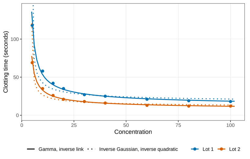
In Figure the inverse-link gamma curves pass through the points, and the inverse-quadratic curves compress too quickly and then flatten too soon.
Now force the inverse Gaussian to use the inverse link, the same mean function as the gamma:
need <- function(pkg) {
  if (!requireNamespace(pkg, quietly = TRUE)) {
    install.packages(pkg, repos = "https://cloud.r-project.org")
  }
  suppressPackageStartupMessages(library(pkg, character.only = TRUE))
}
need("faraway")
data(clot, package = "faraway")
clot$Y <- clot$time
clot$logdose <- log(clot$conc)
clot$lot.f <- factor(clot$lot, levels = c("one", "two"), labels = c("1", "2"))
summary(glm(Y ~ lot.f * logdose, data = clot,
            family = inverse.gaussian(link = "inverse")))
The coefficients come back to -0.0178, -0.0074, 0.0158, 0.0083, close to the gamma fit, with AIC 60.7. The two mean curves lie on top of each other. The standard errors move, because the variance function changed from \phi\mu^2 to \phi\mu^3.
The link chooses the mean curve. The response distribution mainly chooses the standard errors. Those two pieces are essentially orthogonal: you may pair a scientifically sensible link with a distribution that matches the scatter, and neither choice is doing the other’s job.
That separation is what Huang and Rathouz (2017) give in general. It is why families and links can be mixed, and why a worse AIC for the inverse quadratic is a statement about the link, not a mystery of the inverse Gaussian. Other positive families exist and are not in the default glm list: inverse gamma, lognormal, Weibull with the second parameter fixed. A custom family needs a log-likelihood, or, as the next section shows, sometimes only a mean and a variance.
Used in
See also
Gamma regression · Quasi-score and quasi-likelihood · Bids for a bankrupt firm · Quasi-likelihood · Leaf-blotch data · Log link · Inverse link · Variance function