Fisher information
Topic of Introduction to generalised linear models, part of Generalised linear models · Also in Standard errors, and models for counts
Fisher information
| Type | Topic |
| Taught in | Introduction to generalised linear models · Standard errors, and models for counts |
| Part | Generalised linear models |
| Questions using it | 4 |
The expected curvature of the log-likelihood, \mathcal{I}(\theta)=-\mathbb{E}\,\partial^2\ell/\partial\theta\,\partial\theta^\top, which is also the variance of the score. Its inverse approximates the variance of the maximum likelihood estimator, and that is where the standard errors of a GLM come from.
In Introduction to generalised linear models
Fix a current value \boldsymbol{\beta}^{(0)}. Evaluate the mean, the variance and the slope of the mean at that value, and write \mu_i^{(0)}, V_i^{(0)} and \mu'_{(0),i} for those three numbers at observation i. The only unknown left in Equation (11) in Introduction to generalised linear models is the next \boldsymbol{\beta}. Replace the mean by its tangent at the current linear predictor, \mu({\boldsymbol{X}}_i^\top\boldsymbol{\beta}) \approx \mu_i^{(0)}+\mu'_{(0),i}\,{\boldsymbol{X}}_i^\top\bigl(\boldsymbol{\beta}-\boldsymbol{\beta}^{(0)}\bigr). Substitute that approximation into Equation (11) in Introduction to generalised linear models. The equation becomes linear in the unknown step \boldsymbol{\beta}-\boldsymbol{\beta}^{(0)}: \sum_{i=1}^n\frac{y_i-\mu_i^{(0)}}{V_i^{(0)}}\,\mu'_{(0),i}\,{\boldsymbol{X}}_i = \sum_{i=1}^n\frac{\bigl(\mu'_{(0),i}\bigr)^2}{V_i^{(0)}}\,{\boldsymbol{X}}_i{\boldsymbol{X}}_i^\top\bigl(\boldsymbol{\beta}-\boldsymbol{\beta}^{(0)}\bigr). Name the two sides. The working score and the working information at \boldsymbol{\beta}^{(0)} are \begin{align*} {\boldsymbol{U}}^{(0)} &=\sum_{i=1}^n\frac{y_i-\mu_i^{(0)}}{V_i^{(0)}}\,\mu'_{(0),i}\,{\boldsymbol{X}}_i,\\ {\color{blue}\boldsymbol{I}}^{(0)} &=\sum_{i=1}^n\frac{\bigl(\mu'_{(0),i}\bigr)^2}{V_i^{(0)}}\,{\boldsymbol{X}}_i{\boldsymbol{X}}_i^\top. \end{align*} The update is one step of weighted least squares, \boldsymbol{\beta}^{(1)}=\boldsymbol{\beta}^{(0)}+\bigl({\color{blue}\boldsymbol{I}}^{(0)}\bigr)^{-1}{\boldsymbol{U}}^{(0)}. Iterate until \boldsymbol{\beta} stops moving. The matrix {\color{blue}\boldsymbol{I}} is the expected negative Hessian of \ell, which is the Fisher information. The algorithm is Newton–Raphson with that expected second derivative in place of the observed one, and for that reason it is called Fisher scoring. It is the same algorithm for every exponential family we put in the random component. A model outside that class does not inherit it; you would write a separate optimiser.
In Standard errors, and models for counts
For a regular model and a large enough sample, the maximum likelihood estimator \hat{\boldsymbol{\beta}} is asymptotically normal, centred at the true value \boldsymbol{\beta}^\star, with covariance equal to the inverse Fisher information at that true value: \mathrm{cov}(\hat{\boldsymbol{\beta}})\approx {\color{blue}\boldsymbol{I}}(\boldsymbol{\beta}^\star)^{-1}. We never know \boldsymbol{\beta}^\star. The usable matrix plugs in \hat{\boldsymbol{\beta}}: {\color{blue}\boldsymbol{I}}(\hat{\boldsymbol{\beta}}) =\sum_{i=1}^n \frac{\bigl(\mu'({\boldsymbol{X}}_i^\top\hat{\boldsymbol{\beta}})\bigr)^2}{\widehat{\mathrm{Var}}(Y_i)}\, {\boldsymbol{X}}_i{\boldsymbol{X}}_i^\top. The standard error of \hat\beta_j is the square root of the jth diagonal entry of {\color{blue}\boldsymbol{I}}(\hat{\boldsymbol{\beta}})^{-1}. A marginal interval is \hat\beta_j\pm z_{\alpha/2}\,\widehat{\mathrm{se}}(\hat\beta_j). For a GLM we use z, not t. The normal approximation is already a large-sample statement. Once the residual degrees of freedom are past thirty or forty, a t cutoff and 1.96 are not meaningfully different, and the theory that delivers Equation (1) in Standard errors, and models for counts is a central limit theorem, not an exact normal linear model. For 95%, use 1.96.
The estimated coefficients come from Fisher scoring. Their standard errors come from the inverse Fisher information, evaluated at those coefficients. Intervals and tests for a GLM use z, not t.
Cholesterol, with standard errors
Main article: Cholesterol and heart disease
chol_file <- "data/cholest.csv"
if (!file.exists(chol_file)) {
  stop("Could not find data/cholest.csv. Set the working directory to the folder that contains it.")
}
chol <- read.csv(chol_file)
summary(glm(disease ~ gender + cholesterol, data = chol, family = binomial))
summary(glm(disease ~ cholesterol, data = chol, family = binomial))
prints
            Estimate Std. Error z value Pr(>|z|)
(Intercept) -9.3203     2.1714  -4.292  1.77e-05
gender      -0.1094     0.4873  -0.224  0.822
cholesterol  1.5842     0.3836   4.130  3.63e-05
The dispersion is reported as 1. For a binomial, that is a reminder, not an estimate: \mathrm{Var}=p(1-p) exactly, with no free \phi.
Cholesterol has a clear positive association with the log-odds of disease. Sex, given cholesterol, does not: the estimate is a tenth of its standard error. The simpler model drops sex.
            Estimate Std. Error z value Pr(>|z|)
(Intercept) -9.2012     2.0992  -4.383  1.17e-05
cholesterol  1.5549     0.3592   4.329  1.50e-05
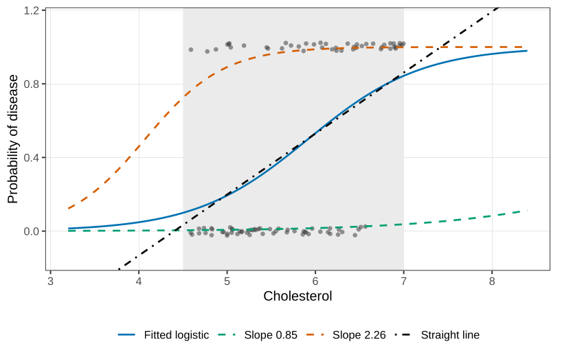
A 95% interval for the cholesterol slope is 1.5549\pm 1.96\times 0.3592=(0.85,\ 2.26). On the odds scale, a one-unit increase in cholesterol multiplies the odds of disease by something between \exp(0.85)=2.34 and \exp(2.26)=9.58. The curve on the probability scale is still an S, flat near 0 and near 1. Drawing the fitted curve at the two endpoints 0.85 and 2.26 is a pointwise band for that single slope. A simultaneous band, allowing the intercept to move as well, is a different object, and it is unnecessary for this one-slope model.
Over the short window from about 4.5 to 7, a straight line and the logistic curve are not dramatically different. That is not a reason to fit the line. A cholesterol of 4.2 or 7.2 would push a straight line outside (0,1). The logistic curve is a valid probability for every cholesterol you might hand it later. If the effect were steeper, the S would be obvious and the line would fail even inside the window. The philosophical objection stands either way.
Used in
- Taught in Introduction to generalised linear models · Standard errors, and models for counts
- Also used in Exponential families and conjugacy · Standard errors, and models for counts · Underdispersion, positive responses, and quasi-likelihood · Mixtures and the EM algorithm
- Questions that use it (4) — Q33 (answer) · Question 19 (answer) · C18 · C19 (answer)
- All 9 questions on Introduction to generalised linear models
See also
Likelihood function · Variance · Maximum likelihood · Standard error · Generalised linear model · Log-partition moment identities · Newton–Raphson method · Score function