Cholesterol and heart disease

Section of Introduction to generalised linear models, part of Generalised linear models · Also in Introduction to generalised linear models, Standard errors, and models for counts

Type	Section
Taught in	Introduction to generalised linear models · Introduction to generalised linear models · Standard errors, and models for counts
Part	Generalised linear models
Questions using it	1

In Introduction to generalised linear models

From Introduction to generalised linear models

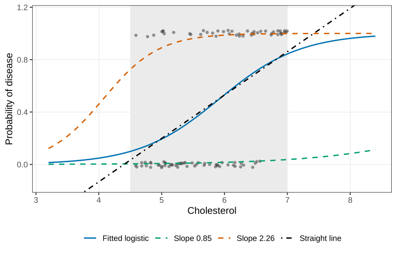
A hundred patients have a cholesterol measurement and a binary disease indicator, with sex marked on the plot. Vertical jitter stops a pile of zeroes, or a pile of ones, looking like a fractional response. The response really is 0 or 1. As cholesterol increases, particularly once it is above about 6.5, disease becomes the typical outcome. Down near 4.5, absence is more common.

The mean of a binary response is the success probability, p=\mathrm{E}(Y\mid {\boldsymbol{X}})=\mathrm{P}(Y=1\mid {\boldsymbol{X}}). A straight line cannot represent it. The line will eventually leave (0,1), and a probability cannot. The exponential \exp({\boldsymbol{X}}^\top\boldsymbol{\beta}) stays positive, but it is not bounded by 1. Dividing by one plus itself fixes that: p=\frac{\exp({\boldsymbol{X}}^\top\boldsymbol{\beta})}{1+\exp({\boldsymbol{X}}^\top\boldsymbol{\beta})} \qquad\text{equivalently}\qquad {\boldsymbol{X}}^\top\boldsymbol{\beta}=\log\frac{p}{1-p}. The right-hand equation is the logistic link, also called the logit: the log of the odds p/(1-p). The left-hand equation is the inverse link, sometimes called the expit. Log-odds run over the whole real line, which is what a linear predictor needs. The probability stays in (0,1).

Again, the link is applied to the mean. The logistic function of a zero or a one is not defined in any useful way, and any function of a binary observation still takes at most two values. You cannot manufacture a curve by transforming zeroes and ones.

The distribution is Bernoulli, a single coin toss, not a normal: Y_i\mid {\boldsymbol{X}}_i\stackrel{\mathrm{ind}}{\sim} \mathrm{Bernoulli}\!\left(p_i=\frac{\exp({\boldsymbol{X}}_i^\top\boldsymbol{\beta})}{1+\exp({\boldsymbol{X}}_i^\top\boldsymbol{\beta})}\right). The variance of a coin toss is p(1-p), so \mathrm{Var}(Y_i\mid {\boldsymbol{X}}_i)=p_i(1-p_i)=\frac{\exp({\boldsymbol{X}}_i^\top\boldsymbol{\beta})}{\bigl(1+\exp({\boldsymbol{X}}_i^\top\boldsymbol{\beta})\bigr)^2}. This variance is not monotone in p. It is largest at p=1/2 and it shrinks towards 0 as p approaches 0 or 1. If almost everyone is diseased, there is little disagreement left in the sample. The same is true if almost nobody is.

Key idea

In all three examples the mean is a function of a linear predictor, and the observations are not transformed. The link is chosen so that the mean stays inside the set of values the response can actually have. The distribution is chosen to match the kind of observation: counts, positive times, or zeroes and ones. The variance formula is then a consequence, not a separate constant \sigma^2.

Put the four models next to each other: \begin{align*} Y_i\mid {\boldsymbol{X}}_i &\stackrel{\mathrm{ind}}{\sim} \mathrm{N}({\boldsymbol{X}}_i^\top\boldsymbol{\beta},\sigma^2),\\ Y_i\mid {\boldsymbol{X}}_i &\stackrel{\mathrm{ind}}{\sim} \mathrm{Poisson}\!\left(\exp({\boldsymbol{X}}_i^\top\boldsymbol{\beta})\right),\\ Y_i\mid {\boldsymbol{X}}_i &\stackrel{\mathrm{ind}}{\sim} \mathrm{Gamma}\!\left(\exp({\boldsymbol{X}}_i^\top\boldsymbol{\beta}),\ \mathrm{Var}=\phi\mu_i^2\right),\\ Y_i\mid {\boldsymbol{X}}_i &\stackrel{\mathrm{ind}}{\sim} \mathrm{Bernoulli}\!\left(\frac{\exp({\boldsymbol{X}}_i^\top\boldsymbol{\beta})}{1+\exp({\boldsymbol{X}}_i^\top\boldsymbol{\beta})}\right). \end{align*} Before Nelder’s work in the early 1970s, each new distribution arrived with its own theory and its own fitting algorithm. These four, and others like them, are exponential families. One piece of theory covers them, and one numerical algorithm fits them.

In Introduction to generalised linear models, continued

From Introduction to generalised linear models

The disease indicator in the third example was fitted, in R, by a logistic regression on sex and cholesterol. Female is the baseline, because the level F comes before M. The fitted log-odds are \log\frac{\hat p}{1-\hat p}=-9.3203-0.1094\,I(\text{male})+1.5842\,(\text{cholesterol}).

The intercept -9.3203 is the log-odds for a female with cholesterol 0. The corresponding probability is \frac{\exp(-9.3203)}{1+\exp(-9.3203)}=8.96\times 10^{-5}. The female half of that baseline is a real category. Cholesterol equal to zero is not a living patient; values below about 4 are already outside anything this sample, or ordinary physiology, is talking about. The number is the correct intercept. It is not a probability to quote in a sentence about these patients.

The cholesterol coefficient 1.5842 is the change in log-odds for a one-unit increase in cholesterol, at fixed sex. On the odds scale that increase multiplies the odds of disease by \exp(1.5842)=4.88. Moving from a cholesterol of 5.5 to 6.5, same sex, is associated with odds of disease about five times larger. The odds may keep growing. The probability cannot, which is why the curve flattens as it approaches 1 and we do not interpret \beta as a change in probability.

The sex coefficient -0.1094 says that, at the same cholesterol, males have log-odds lower by 0.1094 than females, and therefore odds \exp(-0.1094)=0.90 times the odds for a female at that same cholesterol. About 10\% lower. This is the opposite of the crude comparison, and the resolution is the phrase “at the same cholesterol.” Male patients in this kind of study tend to arrive with higher cholesterol. A woman whose cholesterol is 6.5 is further into the upper tail of the female distribution than a man at 6.5 is into his. Comparing them at a common cholesterol value is not the same statement as comparing men and women on average. A paper should not say that males are at lower risk. The sentence to write is that, conditionally on cholesterol, the sex coefficient is small. We will test it properly when we do inference. Ahead of that test, this particular coefficient does not survive it: once cholesterol is in the model, sex is the term expected to drop. The mechanism worth saying out loud is that sex, in this fit, is acting through cholesterol rather than as a separate shift in risk.

In Standard errors, and models for counts

From Standard errors, and models for counts

chol_file <- "data/cholest.csv"
if (!file.exists(chol_file)) {
  stop("Could not find data/cholest.csv. Set the working directory to the folder that contains it.")
}
chol <- read.csv(chol_file)
summary(glm(disease ~ gender + cholesterol, data = chol, family = binomial))
summary(glm(disease ~ cholesterol, data = chol, family = binomial))

prints

            Estimate Std. Error z value Pr(>|z|)
(Intercept) -9.3203     2.1714  -4.292  1.77e-05
gender      -0.1094     0.4873  -0.224  0.822
cholesterol  1.5842     0.3836   4.130  3.63e-05

The dispersion is reported as 1. For a binomial, that is a reminder, not an estimate: \mathrm{Var}=p(1-p) exactly, with no free \phi.

Cholesterol has a clear positive association with the log-odds of disease. Sex, given cholesterol, does not: the estimate is a tenth of its standard error. The simpler model drops sex.

            Estimate Std. Error z value Pr(>|z|)
(Intercept) -9.2012     2.0992  -4.383  1.17e-05
cholesterol  1.5549     0.3592   4.329  1.50e-05

A 95% interval for the cholesterol slope is 1.5549\pm 1.96\times 0.3592=(0.85,\ 2.26). On the odds scale, a one-unit increase in cholesterol multiplies the odds of disease by something between \exp(0.85)=2.34 and \exp(2.26)=9.58. The curve on the probability scale is still an S, flat near 0 and near 1. Drawing the fitted curve at the two endpoints 0.85 and 2.26 is a pointwise band for that single slope. A simultaneous band, allowing the intercept to move as well, is a different object, and it is unnecessary for this one-slope model.

Over the short window from about 4.5 to 7, a straight line and the logistic curve are not dramatically different. That is not a reason to fit the line. A cholesterol of 4.2 or 7.2 would push a straight line outside (0,1). The logistic curve is a valid probability for every cholesterol you might hand it later. If the effect were steeper, the S would be obvious and the line would fail even inside the window. The philosophical objection stands either way.

Figure 1: Probability of disease against cholesterol. Points are jittered off 0 and 1. The shaded window runs from 4.5 to 7. The solid curve is the fitted logistic. The dashed curves keep that intercept and use the endpoints 0.85 and 2.26 of the slope interval. The straight line is least squares, extended until it leaves (0,1).

Used in

Taught in Introduction to generalised linear models · Introduction to generalised linear models · Standard errors, and models for counts
Also used in Standard errors, and models for counts · Paired comparisons, and how far a fit is from the data
Questions that use it (1) — Q35
All 9 questions on Introduction to generalised linear models

In Introduction to generalised linear models

In Introduction to generalised linear models, continued

In Standard errors, and models for counts

Used in

See also