Binary responses in a GLM

Section of Introduction to generalised linear models, part of Generalised linear models

Binary responses in a GLM

Type	Section
Taught in	Introduction to generalised linear models
Part	Generalised linear models
Questions using it	1

A binary GLM is the case for the rest of this chapter. The likelihood is Bernoulli, the same likelihood obtained when the success probability is given a prior; the reading here is frequentist. The response is 0 or 1. The mean is the success probability, and g(p_i)={\boldsymbol{X}}_i^\top\boldsymbol{\beta} for a link g we choose. The Bernoulli distribution handles the zeroes and ones. The covariates, through the inverse link, handle the mean: Y_i\mid {\boldsymbol{X}}_i\stackrel{\mathrm{ind}}{\sim} \mathrm{Bernoulli}\!\left(p_i=\mu({\boldsymbol{X}}_i^\top\boldsymbol{\beta})\right), where \mu=g^{-1}. We work with \mu rather than with g whenever we can.

The same skeleton covers the usual applied questions: whether a firm has an industrial-relations department, as a function of firm size; whether a married woman is in the labour force, as a function of her age, her children, and her husband’s income; whether disease is present, as a function of sex and cholesterol.

Three links

Main article: Logit, probit and complementary log-log links

The logistic link is Equation (5) in Introduction to generalised linear models. It is the link we will interpret, and it is the canonical link.

The probit link replaces the logistic curve by a standard normal distribution function. If \Phi is the cumulative distribution function of \mathrm{N}(0,1), \Phi^{-1}(p_i)={\boldsymbol{X}}_i^\top\boldsymbol{\beta} \qquad\text{equivalently}\qquad p_i=\Phi({\boldsymbol{X}}_i^\top\boldsymbol{\beta}). Read it as a quantile. Compute {\boldsymbol{X}}_i^\top\boldsymbol{\beta}, find that point on the standard normal axis, and take the probability to its left. That left-tail probability is p_i. Any other continuous distribution function would give a link of the same type. The normal is the default.

The complementary log-log link is \log\bigl(-\log(1-p_i)\bigr)={\boldsymbol{X}}_i^\top\boldsymbol{\beta} \qquad\text{equivalently}\qquad p_i=1-\exp\bigl\{-\exp({\boldsymbol{X}}_i^\top\boldsymbol{\beta})\bigr\}. The exercise asks you to check that the right-hand side lies in (0,1) for every real linear predictor. This link is the one that does not treat the two tails symmetrically. Logit and probit both approach 0 and 1 in the same fashion, one a mirror of the other. Complementary log-log can stay near zero for longer and then rise more sharply towards one, or the reverse, depending on the sign of the slope. Use it when that asymmetry is the scientific point. Do not use it because you want a sentence about odds. The coefficient is a log-hazard, an instantaneous risk, and a hazard is much harder to explain to a medical collaborator than an odds ratio.

Figure 1: Three inverse links, each with slope one. The logit and the probit are symmetric about one half. Complementary log-log reaches one faster than it leaves zero.

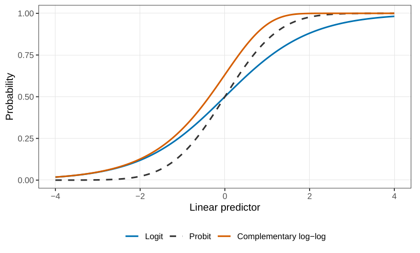
In Figure the logit and the probit differ in the tails and agree through the middle. In a fitted model they almost always agree, close enough that the two curves will not separate. A probit essentially never has to be the link reported to an applied scientist. A log-odds can be explained. A computer scientist or an engineer will sometimes prefer the probit, because a normal quantile is already their language. When there is a choice, and the person across the table is not one of those, use the logit. Goodness of fit will not be the reason to switch.

Interpreting a logistic regression

Main article: Interpreting a logistic regression

Two covariates are enough. If you can say what \beta_1 and \beta_2 mean here, you can say it for twenty: \log\frac{p}{1-p}=\beta_0+\beta_1 x_1+\beta_2 x_2. Hold x_2 fixed and increase x_1 by one unit. The log-odds increase by \beta_1. Equivalently, the odds p/(1-p) are multiplied by e^{\beta_1}. The same sentence with the labels swapped is the interpretation of \beta_2. Log-odds are not a quantity anyone should be expected to feel. Odds are usually as far as a collaborator needs to go: “the odds of disease are multiplied by e^{\beta_1}.”

The intercept is the log-odds when every covariate is zero, and p=\frac{e^{\beta_0}}{1+e^{\beta_0}} is the corresponding probability. That baseline is meaningful only when setting every covariate to zero is a real, or at least a hypothetical, situation. Otherwise it is an algebraically correct description of a point off the edge of the data.

The cholesterol fit

Main article: Cholesterol and heart disease

The disease indicator in the third example was fitted, in R, by a logistic regression on sex and cholesterol. Female is the baseline, because the level F comes before M. The fitted log-odds are \log\frac{\hat p}{1-\hat p}=-9.3203-0.1094\,I(\text{male})+1.5842\,(\text{cholesterol}).

The intercept -9.3203 is the log-odds for a female with cholesterol 0. The corresponding probability is \frac{\exp(-9.3203)}{1+\exp(-9.3203)}=8.96\times 10^{-5}. The female half of that baseline is a real category. Cholesterol equal to zero is not a living patient; values below about 4 are already outside anything this sample, or ordinary physiology, is talking about. The number is the correct intercept. It is not a probability to quote in a sentence about these patients.

The cholesterol coefficient 1.5842 is the change in log-odds for a one-unit increase in cholesterol, at fixed sex. On the odds scale that increase multiplies the odds of disease by \exp(1.5842)=4.88. Moving from a cholesterol of 5.5 to 6.5, same sex, is associated with odds of disease about five times larger. The odds may keep growing. The probability cannot, which is why the curve flattens as it approaches 1 and we do not interpret \beta as a change in probability.

The sex coefficient -0.1094 says that, at the same cholesterol, males have log-odds lower by 0.1094 than females, and therefore odds \exp(-0.1094)=0.90 times the odds for a female at that same cholesterol. About 10\% lower. This is the opposite of the crude comparison, and the resolution is the phrase “at the same cholesterol.” Male patients in this kind of study tend to arrive with higher cholesterol. A woman whose cholesterol is 6.5 is further into the upper tail of the female distribution than a man at 6.5 is into his. Comparing them at a common cholesterol value is not the same statement as comparing men and women on average. A paper should not say that males are at lower risk. The sentence to write is that, conditionally on cholesterol, the sex coefficient is small. We will test it properly when we do inference. Ahead of that test, this particular coefficient does not survive it: once cholesterol is in the model, sex is the term expected to drop. The mechanism worth saying out loud is that sex, in this fit, is acting through cholesterol rather than as a separate shift in risk.

Used in

• Taught in Introduction to generalised linear models
• Also used in Paired comparisons, and how far a fit is from the data · Random slopes, and a binary mixed model · Three species on one hillside
• Questions that use it (1) — Question 20 (answer)
• All 9 questions on Introduction to generalised linear models

See also

Complementary log-log link · Exponential family · Mean and variance of an exponential family · Generalised linear model · Canonical link · What a regression statement is hiding · Three examples the linear model does not fit · Runs in the past week

Glossary and index