Posterior prediction under the reference prior
Theorem taught in Bayesian linear regression, part of Bayesian statistics
Posterior prediction under the reference prior
| Type | Theorem |
| Taught in | Bayesian linear regression |
| Part | Bayesian statistics |
| Worked examples | 1 |
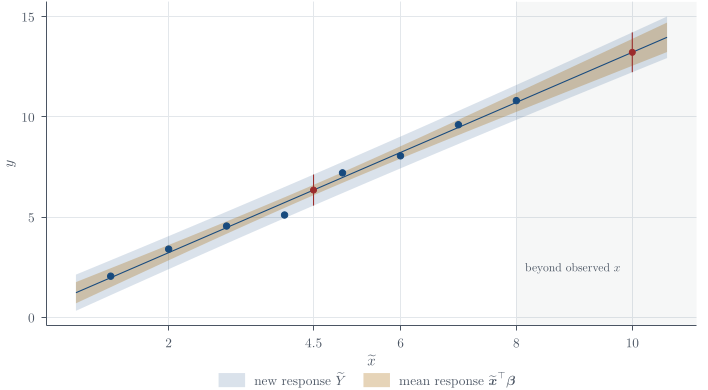
\boxed{ \widetilde Y\mid{\boldsymbol{y}},{\color{blue}\boldsymbol{X}},\widetilde{\boldsymbol{x}} \sim t_{n-p}\!\left( \widetilde{\boldsymbol{x}}^\top\widehat{\boldsymbol{\beta}}, s\sqrt{1+h(\widetilde{\boldsymbol{x}})}\right).} For the unknown mean response itself, there is no new observational error: \widetilde{\boldsymbol{x}}^\top{\boldsymbol{\beta}}\mid{\boldsymbol{y}},{\color{blue}\boldsymbol{X}} \sim t_{n-p}\!\left( \widetilde{\boldsymbol{x}}^\top\widehat{\boldsymbol{\beta}}, s\sqrt{h(\widetilde{\boldsymbol{x}})}\right).
Examples
Q24. Bayesian regression and prediction
Question page: Q24. Bayesian regression and prediction
[12 marks]
Consider the regression model Y_i=\beta_0+\beta_1x_i+\varepsilon_i, \qquad \varepsilon_i\overset{\mathrm{iid}}{\sim}N(0,\sigma^2), with reference prior p(\beta_0,\beta_1,\sigma^2)\propto1/\sigma^2 for (\beta_0,\beta_1)\in\mathbb{R}^2 and \sigma^2>0. For n=10 observations, the design matrix has rows (1,x_i), and \widehat{\boldsymbol\beta}=\begin{pmatrix}1\\2\end{pmatrix}, \qquad (X^\top X)^{-1}=\begin{pmatrix}1/10&0\\0&1/40\end{pmatrix}, \qquad \operatorname{SSE}=16. The observed predictor values range from -3 to 3.
You may use the standard regression posterior formulas under this prior. Use the inverse-Gamma convention f(v)\propto v^{-a-1}e^{-b/v}. Write t_\nu(m,s) for a Student-t distribution with location m and scale s, and use t_{0.975,8}=2.306.
(a) [2 marks] State the marginal posterior distribution of \sigma^2 and calculate \mathbb{E}(\sigma^2\mid\mathbf y,X).
(b) [3 marks] State the marginal posterior distribution of the slope \beta_1, and calculate its equal-tailed 95% credible interval.
(c) [4 marks] At x_*=0, derive the posterior distributions and equal-tailed 95% intervals for:
(i) the unknown mean response \mu_*=\beta_0+\beta_1x_*;
(ii) a new observation \widetilde Y.
Explain precisely why the second interval is wider.
(d) [3 marks] Calculate h(x_*)=(1,x_*)(X^\top X)^{-1}(1,x_*)^\top at x_*=0 and x_*=4. Compare the posterior predictive scales at these points and explain how the calculation reflects uncertainty from extrapolation.
Definitions. Write D=(\mathbf y,X), v=\sigma^2, and \operatorname{SSE}=\|\mathbf y-X\widehat{\boldsymbol\beta}\|^2. The inverse-Gamma kernel is v^{-a-1}e^{-b/v} on v>0. t_\nu(m,s) denotes location m, scale s, and \nu degrees of freedom: (T-m)/s\sim t_\nu. A scale is not a variance; t_{q,\nu} denotes the q quantile of standard t_\nu.
Assumptions. Use independent Normal errors, fixed covariates, full column rank X, n>p, positive SSE, and the reference prior p(\boldsymbol\beta,v)\propto1/v with respect to d\boldsymbol\beta\,dv. These rank and residual conditions ensure a proper posterior despite the improper prior.
There are p=2 regression coefficients, including the intercept. Define \nu=n-p=8,\qquad s^2=\frac{\operatorname{SSE}}{n-p}=\frac{16}{8}=2, \qquad C=(X^\top X)^{-1}. Here s^2 is the residual variance estimate; it is not the posterior mean of \sigma^2.
Why the regression posterior has this form. The likelihood times the reference prior gives p(\boldsymbol\beta,v\mid D) \propto v^{-n/2-1} \exp\{-\|\mathbf y-X\boldsymbol\beta\|^2/(2v)\}, \qquad v=\sigma^2>0. Expand about the least-squares estimate. The cross term vanishes because X^\top(\mathbf y-X\widehat{\boldsymbol\beta})=\mathbf0, giving \|\mathbf y-X\boldsymbol\beta\|^2 =\operatorname{SSE} +(\boldsymbol\beta-\widehat{\boldsymbol\beta})^\top X^\top X(\boldsymbol\beta-\widehat{\boldsymbol\beta}). The second term is a Normal quadratic. At fixed v it identifies \boldsymbol\beta\mid v,D\sim N_p(\widehat{\boldsymbol\beta},vC). Its unnormalised exponential integrates to (2\pi v)^{p/2}|X^\top X|^{-1/2}, which explains the v^{p/2} factor in the variance marginal below.
(a) Marginal variance posterior. Under the stated reference prior, \sigma^2\mid D\sim\operatorname{InvGamma}\left(\frac{n-p}{2}, \frac{\operatorname{SSE}}2\right). Thus \boxed{\sigma^2\mid D\sim\operatorname{InvGamma}(4,8),\qquad\sigma^2>0.} An \operatorname{InvGamma}(a,b) variable has mean b/(a-1) when a>1, so \boxed{\mathbb{E}(\sigma^2\mid D)=\frac8{4-1}=\frac83\approx2.6667.} For completeness, integrating the coefficient kernel out of the joint posterior contributes a factor (\sigma^2)^{p/2}. Therefore p(\sigma^2\mid D) \propto (\sigma^2)^{-(n/2+1)}(\sigma^2)^{p/2} \exp\!\left(-\frac{\operatorname{SSE}}{2\sigma^2}\right) =(\sigma^2)^{-5}e^{-8/\sigma^2}, confirming the shape 4, not n/2=5.
(b) Slope posterior and credible interval. The conditional coefficient posterior is \boldsymbol\beta\mid\sigma^2,D \sim N_2(\widehat{\boldsymbol\beta},\sigma^2 C). The slope entry of C is 1/40, so \beta_1\mid\sigma^2,D\sim N\!\left(2,\frac{\sigma^2}{40}\right). Integrating over \sigma^2\mid D gives \boxed{\beta_1\mid D\sim t_8\!\left(2,\sqrt{\frac2{40}}\right) =t_8(2,\sqrt{0.05}).} Equivalently, (\beta_1-2)/\sqrt{0.05}\mid D\sim t_8. The equal-tailed 95% credible interval is therefore 2\pm2.306\sqrt{0.05}=2\pm0.5156, \qquad\boxed{(1.484,\,2.516).} The second argument of t_8 is a scale, not a variance. There is no additional division by \sqrt n: sample-size information is already in C.
(c) Mean response versus a new observation at x_*=0. For a general predictor value, set \mathbf z_*=(1,x_*)^\top and write m_*=\mathbf z_*^\top\widehat{\boldsymbol\beta}, \qquad h(x_*)=\mathbf z_*^\top C\mathbf z_*. The linear-transformation rule for a normal vector gives \mu_*\mid\sigma^2,D \sim N\bigl(m_*,\sigma^2 h(x_*)\bigr). For a new response \widetilde Y=\mu_*+\widetilde\varepsilon, the new error is independent of the coefficient uncertainty conditional on \sigma^2,D, and has variance \sigma^2. Thus \widetilde Y\mid\sigma^2,D,x_* \sim N\bigl(m_*,\sigma^2\{1+h(x_*)\}\bigr). Integrating over the inverse-Gamma variance posterior gives \mu_*\mid D\sim t_8\bigl(m_*,s\sqrt{h(x_*)}\bigr), \widetilde Y\mid D,x_*\sim t_8\bigl(m_*,s\sqrt{1+h(x_*)}\bigr). At x_*=0, m_*=(1,0)\begin{pmatrix}1\\2\end{pmatrix}=1, \qquad h(0)=\frac1{10}. Therefore the unknown mean response has posterior \boxed{\mu_*\mid D\sim t_8(1,\sqrt{0.2}),} with equal-tailed 95% credible interval 1\pm2.306\sqrt{0.2}=1\pm1.0313, \qquad\boxed{(-0.031,\,2.031).} The new observation has posterior predictive distribution \boxed{\widetilde Y\mid D,x_*=0\sim t_8(1,\sqrt{2.2}),} with equal-tailed 95% predictive interval 1\pm2.306\sqrt{2.2}=1\pm3.4204, \qquad\boxed{(-2.420,\,4.420).} Both intervals have the same centre and use the same t_8 quantile. The predictive interval is wider because a new observation includes both uncertainty about the regression mean and fresh observational noise. That additional noise produces the extra 1 in 1+h(x_*).
(d) Extrapolation and predictive scale. Using the supplied diagonal matrix, \begin{aligned} h(x_*)&=(1,x_*) \begin{pmatrix}1/10&0\\0&1/40\end{pmatrix} \begin{pmatrix}1\\x_*\end{pmatrix}\\ &=\frac1{10}+\frac{x_*^2}{40}. \end{aligned} Hence \boxed{h(0)=0.1,\qquad h(4)=0.1+\frac{16}{40}=0.5.} The corresponding predictive scales are \boxed{s_{\mathrm{pred}}(0)=\sqrt{2(1+0.1)}=\sqrt{2.2}\approx1.4832,} \boxed{s_{\mathrm{pred}}(4)=\sqrt{2(1+0.5)}=\sqrt3\approx1.7321.} At x_*=4, the predicted centre is 1+2(4)=9, so the predictive distribution is t_8(9,\sqrt3). Its interval is wider than at x_*=0 because it has the same degrees of freedom but a larger scale.
The value 4 lies outside the observed range [-3,3]. Uncertainty about the slope has a greater effect on the fitted mean farther from the centred design, increasing h(x_*). The future-error contribution is unchanged; the increased width comes from greater parameter uncertainty in the prediction. This calculation assumes the linear model remains appropriate beyond the observed range; it does not account for possible failure of that model there.
Key result. The mean-response scale is s\sqrt h; the new-observation scale is s\sqrt{1+h}. The extra 1 represents new observational noise, while h measures uncertainty about the fitted mean.
Used in
- Taught in Bayesian linear regression, where the derivation and examples are.
- All 8 questions on Bayesian linear regression
See also
Gaussian linear model · Error and residual · Ordinary least squares · Sampling distribution of the OLS estimator · Studentised coefficient pivot · Least-squares decomposition · Conditional coefficient posterior · Marginal variance posterior