Chi-squared test with estimated parameters
Section of Chi-squared tests, part of Statistical inference
Chi-squared test with estimated parameters
| Type | Section |
| Taught in | Chi-squared tests |
| Part | Statistical inference |
Often the model fixes the form of the cell probabilities but not their values. A count of houses per plot might be Poisson with unknown mean. Then p_i=p_i(\theta) for an unknown r-dimensional parameter \theta, and the expected counts must themselves be estimated.
Theorem 1 (Pearson test with estimated parameters) Let (X_1,\ldots,X_k) be multinomial with cell probabilities p_i(\theta), where \theta has r free coordinates. If \widehat\theta is the maximum likelihood estimator of \theta from the counts and \widehat p_i=p_i(\widehat\theta), then
\sum_{i=1}^k\frac{(X_i-n\widehat p_i)^2}{n\widehat p_i}
is approximately \chi^2_{k-1-r} for large n.
Each freely estimated parameter spends a degree of freedom. The fitted expectations are pulled towards the observed counts by the estimation, so the statistic is smaller than it would be with the true \theta. Using k-1 degrees of freedom anyway, as though \theta were known, makes the test too reluctant to reject.
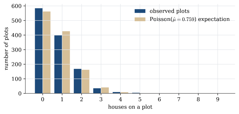
Example 1 (Houses on a village grid) A village of 12 square kilometres is divided into 1200 plots, and the 911 houses are counted plot by plot. If houses are placed at random, the count on a plot should be Poisson.
| Houses on a plot | 0 | 1 | 2 | 3 | 4 | 5 | 6 | 7 | 8 | 9 |
|---|---|---|---|---|---|---|---|---|---|---|
| Plots | 584 | 398 | 168 | 35 | 9 | 4 | 0 | 1 | 0 | 1 |
Question. Test whether the counts per plot are Poisson.
Solution. The maximum likelihood estimate of the Poisson mean is the average count, \widehat\mu=911/1200=0.7592. The fitted expected number of plots with i houses is 1200\,e^{-\widehat\mu}\widehat\mu^{\,i}/i!: 561.67, 426.40, 161.85 and 40.96 for 0 to 3 houses, then 7.77, 1.18 and less than 0.2 after that. To keep every expectation at least 5, merge 4 or more houses into one class, with observed count 15 and expected count 9.12. With k=5 classes and r=1 estimated parameter,
T=\frac{(584-561.67)^2}{561.67}+\frac{(398-426.40)^2}{426.40}+\frac{(168-161.85)^2}{161.85}+\frac{(35-40.96)^2}{40.96}+\frac{(15-9.12)^2}{9.12}=7.67
on 5-1-1=3 degrees of freedom. Since \chi^2_{3;0.95}=7.815, the test just fails to reject at the 5% level; the p-value is 0.053. Most of the statistic comes from the merged tail class: there are more crowded plots, and fewer plots with a single house, than a Poisson law allows. The evidence that houses are not placed at random is suggestive, not conclusive.
Used in
See also
Pearson statistic · Pearson chi-squared approximation · Pearson test with estimated parameters · Chi-squared test of independence · Counts in categories · Chi-squared test with known cell probabilities · Contingency tables · Observed and expected counts