Maximum a posteriori estimate
Topic of Bayesian linear regression, part of Bayesian statistics · Also in Bayesian foundations
Maximum a posteriori estimate
| Type | Topic |
| Taught in | Bayesian linear regression · Bayesian foundations |
| Part | Bayesian statistics |
| Questions using it | 5 |
The posterior mode, \arg\max_\theta p(\theta\mid y). With a flat prior it is the maximum likelihood estimate. In regression a normal prior on the coefficients makes it ridge regression and a Laplace prior makes it the lasso; it keeps none of the posterior’s uncertainty.
In Bayesian linear regression
A centred normal prior also explains ridge regularisation. If \sigma^2 is fixed and {\boldsymbol{\beta}}\sim\operatorname{N}_p({\boldsymbol{0}},\tau^2{\color{blue}\boldsymbol{I}}_p), then \begin{align*} -2\sigma^2\log p({\boldsymbol{\beta}}\mid{\boldsymbol{y}}) &=\operatorname{SSE}({\boldsymbol{\beta}}) +\frac{\sigma^2}{\tau^2}\lVert{\boldsymbol{\beta}}\rVert^2 +\text{a constant}\\ &=\lVert{\boldsymbol{y}}-{\color{blue}\boldsymbol{X}}{\boldsymbol{\beta}}\rVert_2^2 +\frac{\sigma^2}{\tau^2}\lVert{\boldsymbol{\beta}}\rVert_2^2 +\text{the same constant}. \end{align*} The MAP therefore minimises a ridge objective: Euclidean data-space error is balanced against squared Euclidean distance of the coefficient vector from the prior centre, here {\boldsymbol{0}}. A Laplace prior similarly produces an L^1 penalty related to the lasso. MAP keeps only the posterior mode; full Bayes retains coefficient uncertainty and averages predictions over the posterior.
In Bayesian foundations
From Bayesian foundations
Definition 1 (Posterior point summaries) For a scalar parameter, common point summaries include
\mathbb{E}(\theta\mid x)=\int\theta p(\theta\mid x)\,\mathrm{d}\theta, \qquad \widehat\theta_{\mathrm{MAP}} =\operatorname*{arg\,max}_{\theta}p(\theta\mid x),
the posterior median, and posterior quantiles. These summaries need not agree for a skewed distribution.
Definition 2 (Credible-region constructions) Three interval constructions are worth distinguishing. An equal-tailed 95\% credible interval (l,u) satisfies
\mathbb{P}(\theta<l\mid x)=0.025, \qquad \mathbb{P}(\theta>u\mid x)=0.025.
The minimum-width interval solves
\min_{l<u}(u-l) \quad\text{subject to}\quad \int_l^u p(\theta\mid x)\,\mathrm{d}\theta=0.95.
A highest-posterior-density set chooses a level c so that
\mathcal H_c=\{\theta:p(\theta\mid x)\geq c\}, \qquad \int_{\mathcal H_c}p(\theta\mid x)\,\mathrm{d}\theta=0.95.
Every included point then has density at least as large as every excluded point. For a continuous unimodal posterior this gives the minimum-width interval; for a multimodal posterior the highest-density set can be disjoint. For a symmetric unimodal density, the mean, median, and mode coincide and the common interval constructions often agree.
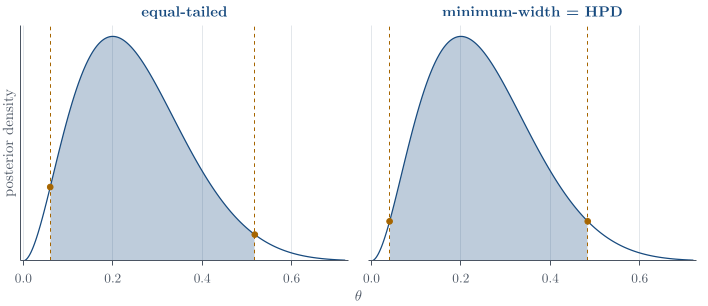
The MAP is a useful point, but a point alone discards the uncertainty that the posterior was introduced to represent. A posterior sample converts most summaries into ordinary sample calculations.
Proposition 1 (Posterior summaries from draws) Let \theta^{(1)},\ldots,\theta^{(L)} be posterior draws and let \theta_{(1)}\leq\cdots\leq\theta_{(L)} be their order statistics. Then \begin{align*} \widehat{\mathbb{E}}(\theta\mid x) &=\frac1L\sum_{l=1}^L\theta^{(l)},\\ \widehat{\operatorname{Var}}(\theta\mid x) &=\frac1{L-1}\sum_{l=1}^L \left(\theta^{(l)}-\overline\theta\right)^2,\\ \widehat{\mathbb{P}}(\theta<c\mid x) &=\frac1L\sum_{l=1}^L\mathbf{1}\{\theta^{(l)}<c\}. \end{align*} The posterior median and equal-tailed interval are estimated by the corresponding empirical quantiles. With L=1000, the median can be estimated by the average of \theta_{(500)} and \theta_{(501)}, and a direct 95\% interval approximation by [\theta_{(25)},\theta_{(975)}]. The precise indices vary slightly with a software package’s quantile convention.
The mode is the exception. It is not an order statistic and, for continuous draws, looking for the most frequently repeated value is generally useless. One should maximise the posterior density or log-posterior, or deliberately construct and optimise a density estimate if the density itself is unavailable.
Remark 1 (R’s distribution interface). For a common distribution, R prefixes the distribution name by d for density, p for cumulative probability, q for quantile, and r for random generation. These are numerical calculations to run once the posterior distribution has been derived. For the \operatorname{Beta}(3,9) posterior in Figure, the following commands compute its median, a posterior probability, an equal-tailed interval, and Monte Carlo versions of the same summaries.
# theta | x ~ Beta(3, 9)
qbeta(0.5, shape1 = 3, shape2 = 9)       # posterior median
pbeta(0.5, shape1 = 3, shape2 = 9)       # P(theta <= 0.5 | x)
qbeta(c(0.025, 0.975), 3, 9)             # equal-tailed interval

set.seed(3500)
theta <- rbeta(1000, shape1 = 3, shape2 = 9)
c(mean = mean(theta),
  median = median(theta),
  Pr_below_half = mean(theta < 0.5))
quantile(theta, c(0.025, 0.975))
The first three lines use the known Beta posterior directly and are preferable when the required function is available. The simulated calculation is the version that survives when the posterior is accessible only through a sampler. Increasing the number of draws reduces Monte Carlo error; it does not repair a sampler that targets the wrong distribution.
Used in
- Taught in Bayesian linear regression · Bayesian foundations
- Also used in Bayesian foundations · The Beta–Binomial model · Markov chains, Gibbs sampling, and Metropolis–Hastings · Categorical data and the Dirichlet distribution · Model selection for stochastic models · Reference formulas and problem-solving workflow
- Questions that use it (5) — Euclidean clusters and mixture components (answer) · Mixtures versus K-means (answer) · Q12 · Q22 · C7
- All 8 questions on Bayesian linear regression
See also
Normal hierarchical shrinkage · Ridge regression · Regularisation · Posterior point summaries · Flat prior · Maximum likelihood · Lasso · Bayesian information criterion