One categorical variable, and two

Section of Descriptive statistics, part of Data analysis

Type	Section
Taught in	Descriptive statistics
Part	Data analysis

A categorical variable is summarised by counts, or by proportions. Of the 299 patients, 96 died during follow-up, a proportion of 0.32.

Two categorical variables are summarised by a contingency table: counts for every combination of categories.

Example 1 (Anaemia and death) Question. Did patients with anaemia die more often?

Solution.

table(heart$anaemia, heart$death, dnn = c("anaemia", "death"))
proportions(table(heart$anaemia, heart$death), margin = 1)

	Survived	Died	Proportion died
No anaemia	120	50	0.294
Anaemia	83	46	0.357

Row proportions, margin = 1, compare the death rate within each anaemia group: 29.4% without anaemia and 35.7% with it. The difference is six percentage points. Whether that is more than chance would produce with groups this size is a chi-squared test of independence, and it is not: the p-value is 0.25. High blood pressure gives 29.4% against 37.1%, with p-value 0.17, while for diabetes, sex and smoking the rates in the two groups differ by less than two percentage points.

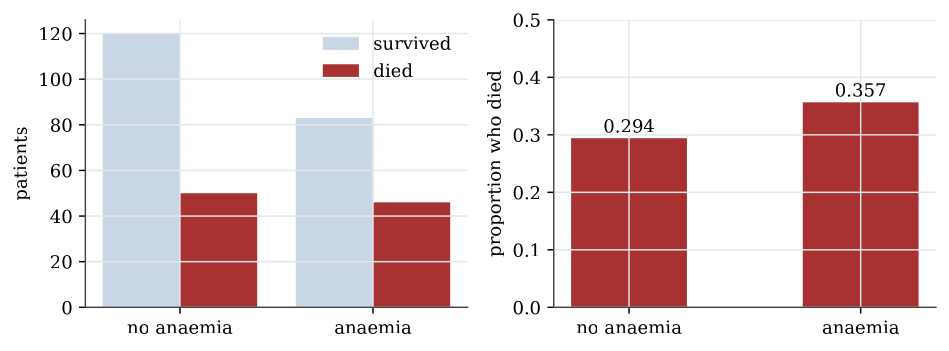
Figure 1: Deaths during follow-up by anaemia status: counts (left) and the proportion who died in each group (right). The counts are hard to compare because the groups differ in size; the proportions are not.

A bar plot shows counts or proportions by bars of proportional length. Side-by-side bars of counts mislead when the groups are of different sizes, which is why the proportions within each group are usually the plot to draw. A pie chart shows the same proportions as angles, which the eye compares less accurately than lengths.

Used in

Taught in Descriptive statistics
All 2 questions on Descriptive statistics

Used in

See also