One quantitative variable
Section of Descriptive statistics, part of Data analysis
One quantitative variable
| Type | Section |
| Taught in | Descriptive statistics |
| Part | Data analysis |
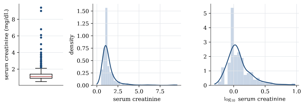
A quantitative variable is summarised by its shape as well as its centre and spread. The serum creatinine levels, a measure of kidney function, show why.
Definition 1 (Five-number summary and boxplot) The five-number summary of a sample is its minimum, first quartile, median, third quartile and maximum. A boxplot draws the box from the first to the third quartile with a line at the median, and whiskers out to the most extreme data within 1.5 interquartile ranges of the box. Points beyond the whiskers are drawn individually as possible outliers.
summary(heart$serum_creatinine)
#  Min. 1st Qu. Median   Mean 3rd Qu.   Max.
#  0.50    0.90   1.10   1.39    1.40   9.40
The mean is pulled above the median by a long right tail: the largest value, 9.4, is more than six times the median. The interquartile range is 1.4-0.9=0.5, so the upper whisker stops at the largest value below 1.4+1.5\times0.5=2.15, and 29 patients lie beyond it.
A histogram counts the data in a set of bins and draws a bar for each; its look depends on the choice of bins. A kernel density estimate smooths the data instead, placing a small bump at each observation and adding them up; its look depends on the width of the bumps, the bandwidth. Both show the same thing here: most patients near 1 mg/dL and a thin tail stretching to 9.
Transformations
Main article: Transformations of data
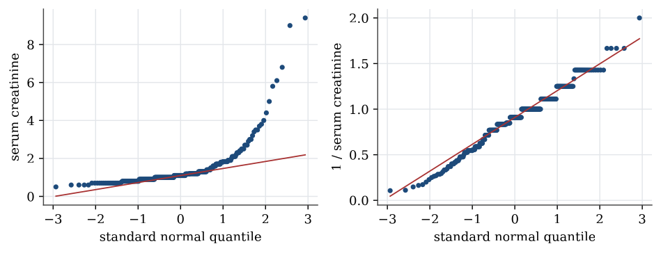
Strongly skewed data are often easier to summarise, and to model, after a transformation. A logarithm turns ratios into differences, so it spreads out the bunched values near zero and draws in the far tail. For serum creatinine the skewness, a measure of asymmetry that is zero for symmetric data, falls from 4.4 to 1.6 on the log scale. The reciprocal, 1/x, brings it to about zero. Transformations do not change the data, only the scale they are viewed on; the order of the patients stays the same, so the median of the transformed data is the transform of the median.
Definition 2 (Normal quantile plot) A normal quantile plot, or Q–Q plot, plots the sorted data against the quantiles of the standard normal distribution at the same fractions. If the data come from a normal distribution, the points lie close to a straight line, whose intercept and slope estimate the mean and standard deviation.
Curvature in a Q–Q plot is how a model check sees skewness. A right-skewed sample bends upwards at the right end; heavy tails bend away from the line at both ends.
Used in
See also
Sample quantile · Interquartile range · Sample variance and standard deviation · Five-number summary and boxplot · Normal quantile plot · Data table · Summary statistics · One categorical variable, and two