Transformations of data
Section of Descriptive statistics, part of Data analysis · Also in Linear model examples
Transformations of data
| Type | Section |
| Taught in | Descriptive statistics · Linear model examples |
| Part | Data analysis |
In Descriptive statistics
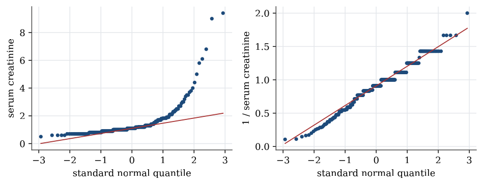
Strongly skewed data are often easier to summarise, and to model, after a transformation. A logarithm turns ratios into differences, so it spreads out the bunched values near zero and draws in the far tail. For serum creatinine the skewness, a measure of asymmetry that is zero for symmetric data, falls from 4.4 to 1.6 on the log scale. The reciprocal, 1/x, brings it to about zero. Transformations do not change the data, only the scale they are viewed on; the order of the patients stays the same, so the median of the transformed data is the transform of the median.
Definition 1 (Normal quantile plot) A normal quantile plot, or Q–Q plot, plots the sorted data against the quantiles of the standard normal distribution at the same fractions. If the data come from a normal distribution, the points lie close to a straight line, whose intercept and slope estimate the mean and standard deviation.
Curvature in a Q–Q plot is how a model check sees skewness. A right-skewed sample bends upwards at the right end; heavy tails bend away from the line at both ends.
In Linear model examples
When the residual plot curves or fans out, a transformation of the response or of an explanatory variable often straightens the relationship and steadies the variance. Common choices are \log y for a response whose spread grows with its mean, \sqrt y for counts, and \log x for an explanatory variable spanning several orders of magnitude. A model for \log y describes multiplicative effects: a unit increase in x multiplies the median of the response by e^\beta, roughly 1+\beta for small \beta. The residual plots are read on the scale that was fitted. Predictions are made on the transformed scale and then transformed back. The melanoma data in Linear regression are an example.
Regression and analysis of variance are the same linear model with different design matrices. A factor enters through indicator columns measured against a reference level; an interaction lets one variable’s slope depend on another; and every coefficient is read with the other variables held fixed.
Used in
- Taught in Descriptive statistics · Linear model examples
- Also used in Linear model examples
- All 2 questions on Descriptive statistics
See also
Sample quantile · Interquartile range · Sample variance and standard deviation · Five-number summary and boxplot · Normal quantile plot · Data table · Summary statistics · One categorical variable, and two