Regression effect
Section of Linear regression, part of Statistical inference
Regression effect
| Type | Section |
| Taught in | Linear regression |
| Part | Statistical inference |
Regression analysis explains a response variable by one or more explanatory variables. The name comes from Francis Galton, who noticed in the 1880s that the children of unusually tall parents are, on the whole, less unusually tall. A father 5% taller than average tends to have a son less than 5% taller than average. Galton called it regression towards mediocrity.
Picture the heights of about a thousand fathers and their adult sons, with the fathers averaging 67 inches and the sons 68 inches. Since sons are one inch taller on average, it is tempting to predict a son’s height as his father’s plus one inch, the line y=x+1. Look at the fathers near 63 inches: most of their sons lie above that line. Near 71 inches, most lie below it. The line through the middle of each vertical strip has slope less than one. That is the regression effect, and finding that line is the job of least squares.
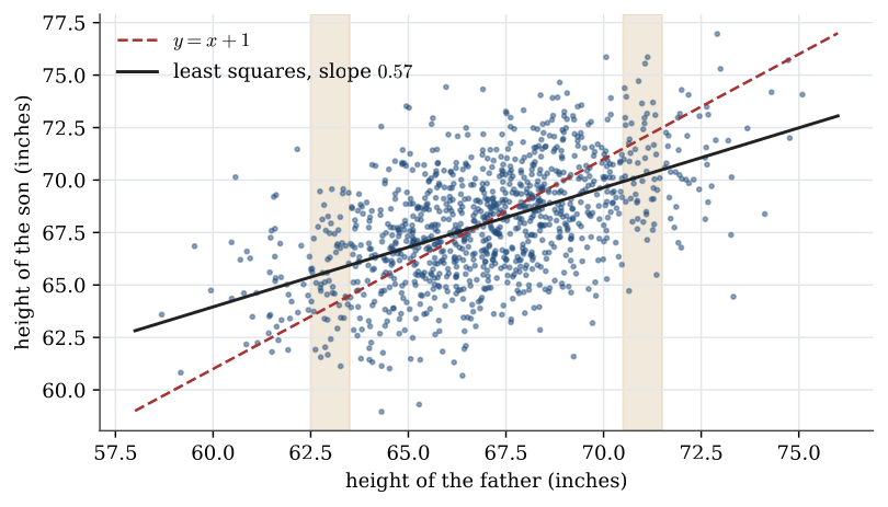
The effect is not a force pulling families towards the mean. When two variables have the same spread and correlation \rho<1, the best linear prediction of one from the other moves only a fraction \rho of the way. Predicting fathers from sons shows the same regression in reverse.
Used in
See also
Least-squares line · Least-squares estimators are unbiased · Simple linear regression · Sampling distribution of the regression estimators · Slope t pivot · Coefficient of determination · Prediction interval · Least squares