Binomial counts in a GLM

Section of Standard errors, and models for counts, part of Generalised linear models

Type	Section
Taught in	Standard errors, and models for counts
Part	Generalised linear models

Often we do not record a zero or a one for every beetle, patient, or firm. We apply a treatment to a group and count the successes. Group sizes need not match. If the members of a group are independent, the likelihood is the Bernoulli likelihood multiplied by a binomial coefficient that does not depend on \boldsymbol{\beta}. The maximiser is unchanged. The data can be stored as two columns, successes and failures, and glm recognises that layout.

Bliss (1935) exposed beetles to carbon disulphide for five hours. The dose on the page is already \log_{10} of concentration, so one unit is a tenfold increase.

\log_{10} dose	beetles n_i	killed y_i
1.6907	59	6
1.7242	60	13
1.7552	62	18
1.7842	56	28
1.8113	63	52
1.8369	59	53
1.8610	62	61
1.8839	60	60

dose <- c(1.6907, 1.7242, 1.7552, 1.7842, 1.8113, 1.8369, 1.8610, 1.8839)
killed <- c(6, 13, 18, 28, 52, 53, 61, 60)
notkilled <- c(53, 47, 48, 28, 11, 6, 1, 0)
response <- cbind(killed, notkilled)
summary(glm(response ~ dose, family = binomial))

The fit, in four Fisher-scoring iterations, is

            Estimate Std. Error z value Pr(>|z|)
(Intercept)  -61.249      5.206  -11.76   <2e-16
dose           34.555      2.926   11.81   <2e-16

A coefficient of 34.6 per unit of \log_{10} dose is a statement about a tenfold change in concentration, and the experiment only runs from 1.69 to 1.88.

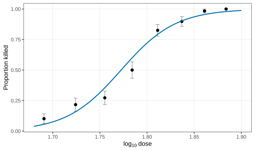
Figure 1: Proportion of beetles killed against log dose, with binomial standard errors. One unit on the horizontal axis is a tenfold change in concentration. The experiment covers only the short stretch drawn here.

Quoting a one-unit effect is like quoting a one-kilometre effect in a study of human height. Bring the unit back to the data. For an increase of 0.01 in log-dose, \exp(0.3456)=1.41, so the odds of being killed are multiplied by about 1.41. The standard error scales the same way, 2.926\times 0.01=0.02926, and \begin{align*} \exp(0.3456-1.96\times 0.02926)&=\exp(0.288)=1.33,\\ \exp(0.3456+1.96\times 0.02926)&=\exp(0.403)=1.50. \end{align*} Rounding can put the upper endpoint at 1.49 rather than 1.50. Either rounding is the same scientific sentence: a small step up in log-dose raises the odds of death by roughly 30 to 50 percent, and the interval sits entirely above 1.

Binomial counts in a GLM

Used in

See also