Standard errors in a GLM
Section of Standard errors, and models for counts, part of Generalised linear models
Standard errors in a GLM
| Type | Section |
| Taught in | Standard errors, and models for counts |
| Part | Generalised linear models |
For a regular model and a large enough sample, the maximum likelihood estimator \hat{\boldsymbol{\beta}} is asymptotically normal, centred at the true value \boldsymbol{\beta}^\star, with covariance equal to the inverse Fisher information at that true value: \mathrm{cov}(\hat{\boldsymbol{\beta}})\approx {\color{blue}\boldsymbol{I}}(\boldsymbol{\beta}^\star)^{-1}. We never know \boldsymbol{\beta}^\star. The usable matrix plugs in \hat{\boldsymbol{\beta}}: {\color{blue}\boldsymbol{I}}(\hat{\boldsymbol{\beta}}) =\sum_{i=1}^n \frac{\bigl(\mu'({\boldsymbol{X}}_i^\top\hat{\boldsymbol{\beta}})\bigr)^2}{\widehat{\mathrm{Var}}(Y_i)}\, {\boldsymbol{X}}_i{\boldsymbol{X}}_i^\top. The standard error of \hat\beta_j is the square root of the jth diagonal entry of {\color{blue}\boldsymbol{I}}(\hat{\boldsymbol{\beta}})^{-1}. A marginal interval is \hat\beta_j\pm z_{\alpha/2}\,\widehat{\mathrm{se}}(\hat\beta_j). For a GLM we use z, not t. The normal approximation is already a large-sample statement. Once the residual degrees of freedom are past thirty or forty, a t cutoff and 1.96 are not meaningfully different, and the theory that delivers Equation (1) in Standard errors, and models for counts is a central limit theorem, not an exact normal linear model. For 95%, use 1.96.
The estimated coefficients come from Fisher scoring. Their standard errors come from the inverse Fisher information, evaluated at those coefficients. Intervals and tests for a GLM use z, not t.
Cholesterol, with standard errors
Main article: Cholesterol and heart disease
chol_file <- "data/cholest.csv"
if (!file.exists(chol_file)) {
  stop("Could not find data/cholest.csv. Set the working directory to the folder that contains it.")
}
chol <- read.csv(chol_file)
summary(glm(disease ~ gender + cholesterol, data = chol, family = binomial))
summary(glm(disease ~ cholesterol, data = chol, family = binomial))
prints
            Estimate Std. Error z value Pr(>|z|)
(Intercept) -9.3203     2.1714  -4.292  1.77e-05
gender      -0.1094     0.4873  -0.224  0.822
cholesterol  1.5842     0.3836   4.130  3.63e-05
The dispersion is reported as 1. For a binomial, that is a reminder, not an estimate: \mathrm{Var}=p(1-p) exactly, with no free \phi.
Cholesterol has a clear positive association with the log-odds of disease. Sex, given cholesterol, does not: the estimate is a tenth of its standard error. The simpler model drops sex.
            Estimate Std. Error z value Pr(>|z|)
(Intercept) -9.2012     2.0992  -4.383  1.17e-05
cholesterol  1.5549     0.3592   4.329  1.50e-05
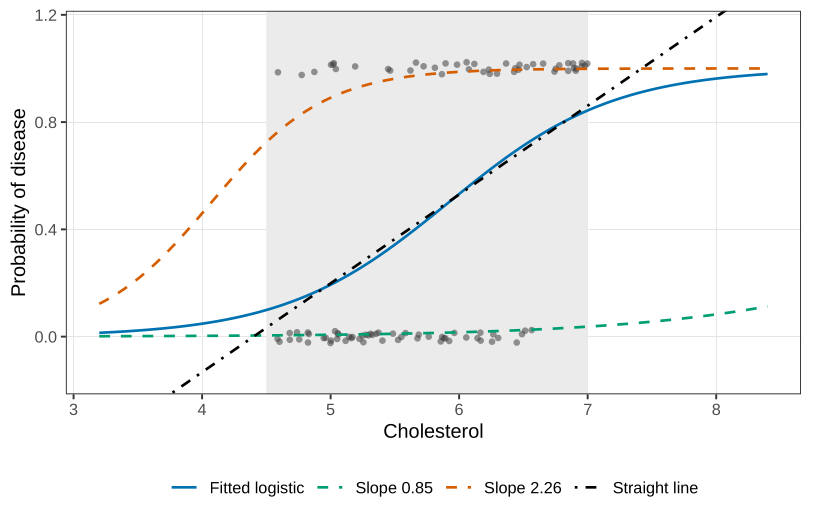
A 95% interval for the cholesterol slope is 1.5549\pm 1.96\times 0.3592=(0.85,\ 2.26). On the odds scale, a one-unit increase in cholesterol multiplies the odds of disease by something between \exp(0.85)=2.34 and \exp(2.26)=9.58. The curve on the probability scale is still an S, flat near 0 and near 1. Drawing the fitted curve at the two endpoints 0.85 and 2.26 is a pointwise band for that single slope. A simultaneous band, allowing the intercept to move as well, is a different object, and it is unnecessary for this one-slope model.
Over the short window from about 4.5 to 7, a straight line and the logistic curve are not dramatically different. That is not a reason to fit the line. A cholesterol of 4.2 or 7.2 would push a straight line outside (0,1). The logistic curve is a valid probability for every cholesterol you might hand it later. If the effect were steeper, the S would be obvious and the line would fail even inside the window. The philosophical objection stands either way.
Used in
See also
Binomial counts in a GLM · Count responses · Quasi-Poisson · Reading a log-linear coefficient · Mine-injury data · Count models beyond the Poisson · Overdispersion · Underdispersion