Coverage
Section of Confidence intervals, part of Statistical inference
Coverage
| Type | Section |
| Taught in | Confidence intervals |
| Part | Statistical inference |
Definition 1 (Confidence interval) Let L and U be statistics. The random interval (L,U) is a confidence interval for \theta with confidence 1-\alpha when
\mathbb{P}_\theta(L<\theta<U)=1-\alpha
for every \theta. A one-sided interval leaves one endpoint infinite.
The observed interval (l,u), computed from the data, is still called the confidence interval. Smaller \alpha means a wider interval, and a very wide interval says little. The usual choices are 0.01, 0.05 and 0.10, that is 99%, 95% and 90% confidence. When the coverage holds only for large samples, the interval is approximate.
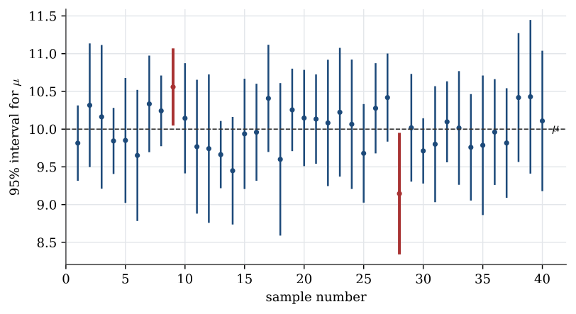
The confidence interval laboratory repeats the interval on fresh samples from a known population, marks the ones that miss, and sets that running fraction next to the coverage the formula claims.
Suppose a 90% interval for \mu comes out as (9.5,10.5). It is tempting to write \mathbb{P}(9.5<\mu<10.5)=0.9, but \mu is a fixed number, so that probability is either 0 or 1, and which one is unknown. The 0.9 belongs to the random interval (L,U) before the data arrive. An urn holds 90 white balls and 10 black. Draw one without looking. You are fairly sure it is white, and you hold it in a closed hand. That is the right degree of confidence that (9.5,10.5) contains \mu.
Definition 2 (Pivot) A pivot is a function h({\boldsymbol{X}};\theta) of the data and the parameter whose distribution does not depend on any unknown parameter.
Every interval in this chapter is built the same way. Find a pivot. Choose its quantiles h_{\alpha/2} and h_{1-\alpha/2}, so that
\mathbb{P}\bigl(h_{\alpha/2}<h({\boldsymbol{X}};\theta)<h_{1-\alpha/2}\bigr)=1-\alpha.
Rearrange the inequality to isolate \theta. The rearrangement does not change the event, so the coverage is still 1-\alpha. The pivot must not depend on unknown parameters, or its quantiles cannot be computed. That is why the t statistic, which replaces \sigma by s, is a pivot, and \sqrt n(\overline X-\mu)/\sigma with unknown \sigma is not.
Used in
See also
Confidence interval · Pivot · One-sample t pivot · Pooled variance · Two-sample t pivot · Variance-ratio F pivot · Wald interval · Interval for a normal variance