Two-factor analysis of variance
Intermediate
One factor splits a sample into groups. Two factors cross those groups, and the mean may depend on each factor separately or on their combination.
What you need first. Read Analysis of variance.
Part of Statistical inference · 2 questions on this topic · What links here
Two-factor analysis of variance
| Part | Statistical inference |
| Level | Intermediate |
| Chapter | 15 of 16 in this part |
| Previous | Linear hypotheses |
| Next | Predictive values of a test |
| Questions | 2 |
| Figures | 1 |
One factor splits a sample into groups. Two factors cross those groups: every level of the first is observed with every level of the second. The mean may depend on each factor separately, and it may depend on the combination. The second possibility is an interaction. The F tests are linear hypotheses in the normal linear model, one for the interaction and one for each main effect.
The one-factor geometry and the randomised block design, which is a two-factor layout with one observation per cell and no interaction term, are in Analysis of variance. Fitting the same models and reading an interaction plot in R, on a larger experiment, is in Analysis of variance examples. This page derives the constraints and works a complete numerical example.
Two-factor analysis of variance
Main article: Two-factor analysis of variance
Index the first factor by j=1,\ldots,J, the second by k=1,\ldots,K, and the replicate by i=1,\ldots,n_{jk}. The model with interaction is
Y_{jki}=\mu+\alpha_j+\beta_k+\gamma_{jk}+\varepsilon_{jki},
with the errors independent \operatorname{N}(0,\sigma^2). Here \alpha_j is a main effect of the first factor, \beta_k a main effect of the second, and \gamma_{jk} the interaction. There is no interaction when every \gamma_{jk}=0. In that additive model the difference between two levels of the first factor is the same at every level of the second.
The parameters as written are not identifiable. Adding a constant to every \alpha_j and subtracting it from \mu does not change a single mean. The same is true of the \beta_k, and an interaction table has the corresponding additions along its rows and columns. A model with 1+J+K+JK symbols is being asked to describe JK cell means. Constraints remove the extra symbols. Two conventions are used.
The sum-to-zero constraints set
\sum_{j=1}^J\alpha_j=0, \qquad \sum_{k=1}^K\beta_k=0, \qquad \sum_{j=1}^J\gamma_{jk}=0\text{ for each }k, \qquad \sum_{k=1}^K\gamma_{jk}=0\text{ for each }j.
Then \mu is a grand mean, \alpha_j is a deviation from it, and \gamma_{jk} is the part of the cell mean left after both main effects. They are comfortable for a balanced experiment in which no level is a control.
The contrast constraints, also called treatment or corner-point constraints, set the first level of each factor to zero:
\alpha_1=0, \qquad \beta_1=0, \qquad \gamma_{1k}=\gamma_{j1}=0.
Then \mu is the mean of the reference cell (j,k)=(1,1). The remaining parameters are changes from that cell:
- \alpha_j is the change in mean when the first factor moves from level 1 to level j, with the second factor held at its reference level;
- \beta_k is the change when the second factor moves from level 1 to level k, with the first factor held at its reference level;
- \gamma_{jk} is the extra change when both factors move, beyond the sum of the two separate changes.
R uses the contrast constraints. The coefficients in lm are these changes, and a coefficient is meaningless without the reference level it is measured from. The sum-to-zero version describes the same cell means. It does not describe the same numerical coefficients. A test of “no interaction” is H_0:\gamma_{jk}=0 for every j,k that the constraints leave free, and that hypothesis does not depend on which constraints were used. A test of a single printed coefficient does.
The cell means determine the sums of squares. Write \overline Y_{jk\cdot} for a cell mean, \overline Y_{j\cdot\cdot} for a level of the first factor, \overline Y_{\cdot k\cdot} for a level of the second, and \overline Y_{\cdot\cdot\cdot} for the grand mean. With n observations in every cell,
\begin{aligned} \mathrm{SS}_A&=nK\sum_j(\overline Y_{j\cdot\cdot}-\overline Y_{\cdot\cdot\cdot})^2,\\ \mathrm{SS}_B&=nJ\sum_k(\overline Y_{\cdot k\cdot}-\overline Y_{\cdot\cdot\cdot})^2,\\ \mathrm{SS}_{AB}&=n\sum_j\sum_k(\overline Y_{jk\cdot}-\overline Y_{j\cdot\cdot}-\overline Y_{\cdot k\cdot}+\overline Y_{\cdot\cdot\cdot})^2,\\ \mathrm{SS}_E&=\sum_j\sum_k\sum_i(Y_{jki}-\overline Y_{jk\cdot})^2. \end{aligned}
The term inside \mathrm{SS}_{AB} is the interaction residual of the cell mean. It is zero for every cell when the cell means are additive. The degrees of freedom are J-1, K-1, (J-1)(K-1) and nJK-JK. The mean squares divide by those degrees of freedom, and each F statistic divides a mean square by the error mean square. Under the normal model and the corresponding null hypothesis, the three numerators are independent of the error and the ratios are F.
Testing the interaction uses (J-1)(K-1) and JK(n-1) degrees of freedom. With one observation per cell, n=1, the error sum of squares is zero once the interaction is fitted, and the interaction cannot be tested. That is why a randomised block design assumes additivity and uses the interaction row as the error.
These F statistics are the general linear hypothesis for three choices of R. No interaction is the set of restrictions \gamma_{jk}=0. No main effect of the first factor, in the presence of interaction, is a restriction on the \alpha_j after the coding constraints, and it is often the wrong restriction to read: if the effect of the first factor changes with the second, a single main-effect mean square averages over that change. The cell means are the summary. The main-effect test is the useful one when the interaction is absent, or small enough that an average effect is the quantity the experiment was built to estimate.
Sum-to-zero and contrast constraints
Main article: Sum-to-zero and contrast constraints
Eight pots carry a crossed experiment: fertiliser at two levels, water at two levels, two pots in each cell.
| Dry | Wet | |
|---|---|---|
| Low fertiliser | 4, 6 | 7, 9 |
| High fertiliser | 6, 8 | 14, 16 |
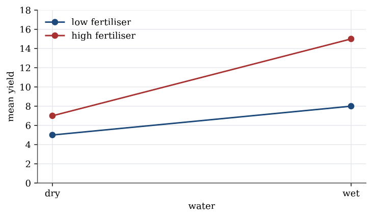
The cell means are 5, 8, 7 and 15. The grand mean is 8.75. Low fertiliser averages 6.5 and high fertiliser averages 11. Dry averages 6 and wet averages 11.5.
The sums of squares, with n=2, J=K=2, are
\begin{aligned} \mathrm{SS}_{\mathrm{fert}}&=4\bigl\{(6.5-8.75)^2+(11-8.75)^2\bigr\}=40.5,\\ \mathrm{SS}_{\mathrm{water}}&=4\bigl\{(6-8.75)^2+(11.5-8.75)^2\bigr\}=60.5,\\ \mathrm{SS}_{\mathrm{int}}&=2\bigl\{(5-6.5-6+8.75)^2+\cdots\bigr\}=12.5,\\ \mathrm{SS}_E&=(4-5)^2+(6-5)^2+\cdots+(16-15)^2=8. \end{aligned}
Each main effect has 1 degree of freedom, the interaction has 1, and the error has 4. The error mean square is 8/4=2. The F statistics are 40.5/2=20.25, 60.5/2=30.25 and 12.5/2=6.25, with upper-tail probabilities 0.011, 0.005 and 0.067. The upper 5\% point of F_{1,4} is 7.71. Both main effects are large. The interaction is the pattern in the table, an increase of 3 when water is added at low fertiliser and an increase of 8 at high fertiliser, and F=6.25 does not clear 7.71. With two pots per cell the experiment can see the pattern and cannot yet call it significant at 5\%. That is a statement about residual degrees of freedom, not a statement that the cell means are additive. The lines on the interaction plot are not parallel. The test says the non-parallelism is still compatible with additive means plus the noise in these eight pots.
Read the same means under contrast constraints, with low fertiliser and dry water as the reference cell. The reference mean is \mu=5. Moving to high fertiliser, still in dry conditions, changes the mean by \alpha_{\mathrm{high}}=7-5=2. Moving to wet conditions, still at low fertiliser, changes the mean by \beta_{\mathrm{wet}}=8-5=3. The high-and-wet cell is 15, which is 5+2+3 plus an extra \gamma=5. The interaction coefficient is the gap between the two water effects, 8-3=5. Under sum-to-zero constraints the interaction is the same scientific fact and a different number, because each coefficient is then a deviation from an average rather than a change from the dry, low cell.
yield <- c(4, 6, 7, 9, 6, 8, 14, 16)
fert <- factor(rep(c("low", "high"), each = 4), levels = c("low", "high"))
water <- factor(rep(c("dry", "wet"), each = 2, times = 2), levels = c("dry", "wet"))
anova(lm(yield ~ fert * water))
# Coefficients are the contrast-constraint parameters, reference low/dry:
coef(lm(yield ~ fert * water))
# mu = 5, alpha_high = 2, beta_wet = 3, gamma = 5
If the interaction is dropped, the additive fit yield ~ fert + water pools \mathrm{SS}_{\mathrm{int}} into the error. The new error sum of squares is 12.5+8=20.5 on 5 degrees of freedom, and the main-effect F statistics are recomputed with that larger error mean square. Pooling is reasonable when the interaction F is small and the scientific question is an average fertiliser effect. It is not reasonable when the lines cross so sharply that the average hides the cell that actually matters. The crop example on the data-analysis page is that second situation: the interaction F is enormous, and the report is the table of cell means rather than a single fertiliser coefficient.
A significant interaction also changes what a main-effect coefficient means. Under the contrast constraints, \alpha_{\mathrm{high}}=2 is the fertiliser effect in dry conditions only. It is not the fertiliser effect averaged over water, and it is not the fertiliser effect in the wet. Quoting it as “the effect of fertiliser” drops the condition that makes the number true.
Two factors need a constraint before their coefficients mean anything. Contrast constraints measure every change from a reference cell, and the interaction is the extra change when both factors leave that cell. Sum-to-zero constraints measure deviations from averages. The F test for no interaction is the same hypothesis either way. When that test is not small, read the cell means. The main-effect coefficients are changes at the reference, or averages, and neither one is the whole experiment.
Questions on this topic
Open a question to attempt it. Its worked answer is folded away at the bottom of the page.
2 questions.
| Question | Level | Answer |
|---|---|---|
| Read the reference cell | Intermediate | ✓ |
| An interaction sum of squares | Intermediate | ✓ |
What links here
Pages (5)
- Statistical inference — via two-factor analysis of variance
- Analysis of variance — via two-factor analysis of variance
- Linear hypotheses — via two-way analysis of variance, Two-factor analysis of variance
- Analysis of variance examples — via Two-factor analysis of variance
- Using R — via Two-factor analysis of variance