Predictive values of a test
Intermediate
Sensitivity and specificity describe a test conditional on the truth. The predictive values run the other way: the chance the condition is present given the test result, which depends on how common the condition is.
What you need first. Read Hypothesis tests and Studies, data, and evidence.
Part of Statistical inference · 2 questions on this topic · What links here
Predictive values of a test
| Part | Statistical inference |
| Level | Intermediate |
| Chapter | 16 of 16 in this part |
| Previous | Two-factor analysis of variance |
| Questions | 2 |
| Figures | 1 |
Sensitivity and specificity describe a test conditional on the truth. Sensitivity is the probability the test is positive when the condition is present. Specificity is the probability the test is negative when the condition is absent. Neither one is the probability the condition is present given a positive test. That reversed probability is the positive predictive value, and it depends on how common the condition is. Confusing the two directions is the fallacy of the transposed conditional.
On a confusion matrix these are row proportions and column proportions. The matrix and the names sensitivity and specificity are on Estimating error rates. The type I and type II errors of a hypothesis test are the same two conditional probabilities, with the null playing the role of “condition absent”. This page is the Bayes calculation that turns them back into a probability for the condition.
Positive predictive value
Main article: Positive predictive value
Let D be the event that the condition is present, and let T+ be the event that the test is positive. Write p_1=\mathbb{P}(D) for the prevalence and p_0=1-p_1. In the language of a hypothesis test, take H_0 to be “the condition is absent” and H_1 to be “the condition is present”, and write \alpha for the probability of a positive test when the condition is absent and \beta for the probability of a negative test when it is present. Then
\text{sensitivity}=1-\beta=\mathbb{P}(T+\mid D), \qquad \text{specificity}=1-\alpha=\mathbb{P}(T-\mid D^c).
The positive predictive value is
\mathrm{PPV}=\mathbb{P}(D\mid T+)=\frac{p_1(1-\beta)}{p_1(1-\beta)+p_0\alpha}.
In prior odds R=p_1/p_0 the same quantity is
\mathrm{PPV}=\frac{1-\beta}{(1-\beta)+R^{-1}\alpha}.
The formula is Bayes’ theorem. Nothing in it requires the test to be a medical assay. D can be “the parameter lies in the alternative” and T+ can be “the level-\alpha test rejects”, in which case 1-\beta is the power and the PPV is the probability the alternative is true given a rejection. That reading needs a prior probability for the alternative. A p-value does not supply one.
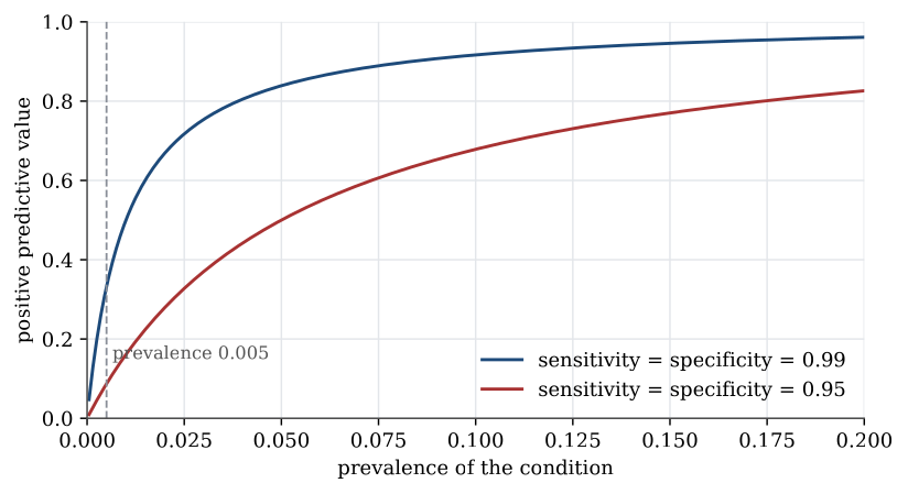
A screening test can be very sensitive and still have a small PPV. Suppose the test has sensitivity 0.95 and specificity 0.95, so \alpha=\beta=0.05, and the prevalence is p_1=0.005. Then
\mathrm{PPV}=\frac{0.005\times 0.95}{0.005\times 0.95+0.995\times 0.05}=\frac{0.00475}{0.0545}=0.087.
About 91\% of the positive tests are false alarms. The test is not broken. The condition is rare, so the many true negatives produce more false positives than the few true cases produce true positives. Raising the sensitivity and the specificity to 0.99 does not remove the problem when R=10^{-3}:
\mathrm{PPV}=\frac{0.99}{0.99+10^3\times 0.01}=\frac{0.99}{10.99}=0.090.
If the prior odds rise to R=10^{-2}, the same test has \mathrm{PPV}=0.99/(0.99+1)=0.497. Prevalence, not the second decimal place of the sensitivity, is what moves the PPV in a rare condition.
The threshold that defines a positive test trades sensitivity against specificity. A low threshold catches more cases and raises 1-\beta, and it also raises \alpha. A screening programme that must not miss a case sets the threshold so that the sensitivity is close to one, accepts a large \alpha, and applies a second, more specific test only to the positives. The PPV of the first test is then deliberately allowed to be modest. The PPV of the two-test sequence is the quantity that matters, and it is computed from the joint event “both tests positive”.
There is a reporting version of the same formula. Suppose a negative result is written up as a positive result with probability u, whether or not the condition is present, and a genuinely positive result is always reported. Then
\mathbb{P}(\text{reported positive}\mid D)=(1-\beta)+u\beta, \qquad \mathbb{P}(\text{reported positive}\mid D^c)=\alpha+u(1-\alpha),
and the PPV of a reported positive replaces 1-\beta and \alpha in the Bayes formula by those two mixtures. The bias u is not sampling noise. Sampling noise is already in \alpha and \beta. The bias is a systematic misreporting of the sign. Any u>0 moves false results into the reported-positive pile and lowers the PPV.
Repeating an independent test changes the odds in the other direction. If n independent tests must all be positive, and each has the same sensitivity and specificity, the likelihood ratio of that joint event is \{(1-\beta)/\alpha\}^n. The posterior odds are R times that ratio. Whenever 1-\beta>\alpha, the ratio exceeds one and the posterior odds tend to infinity with n, so the PPV of the joint positive result tends to 1. One significant result is a single factor (1-\beta)/\alpha. A procedure that rarely fails to repeat is a power of that factor. The PPV of an unreplicated result can stay low because R is low. The PPV of a result that survives several independent repetitions does not.
# PPV from prevalence, sensitivity and specificity.
ppv <- function(prevalence, sensitivity, specificity) {
  p1 <- prevalence
  alpha <- 1 - specificity
  beta <- 1 - sensitivity
  p1 * (1 - beta) / (p1 * (1 - beta) + (1 - p1) * alpha)
}
ppv(0.005, 0.95, 0.95)    # 0.0872
ppv(0.001 / 1.001, 0.99, 0.99)  # prior odds 0.001, about 0.090
Negative predictive value
Main article: Negative predictive value
The negative predictive value is the probability the condition is absent given a negative test,
\mathrm{NPV}=\mathbb{P}(D^c\mid T-)=\frac{p_0(1-\alpha)}{p_0(1-\alpha)+p_1\beta}=\frac{1-\alpha}{(1-\alpha)+R\beta}.
For the screening test with sensitivity and specificity 0.95 and prevalence 0.005,
\mathrm{NPV}=\frac{0.995\times 0.95}{0.995\times 0.95+0.005\times 0.05}=\frac{0.94525}{0.9455}=0.9997.
A negative result is very trustworthy precisely because the condition is rare and the test does not miss many cases. The asymmetry with the PPV is the point of keeping the two names. A test can be trusted when it says “absent” and not trusted when it says “present”, or the reverse if the condition is common and the sensitivity is poor. Reporting only the sensitivity describes neither of those decisions.
The same split is why a small p-value and a large p-value are not mirror images in a rare-effect setting. A rejection can still be a false rejection if most hypotheses tested are null. A non-rejection, when the power is decent and the effect would have mattered, is stronger evidence for the null than the PPV analogy suggests only if the prior odds are not already tiny. The formula, not the surprise, decides which way the asymmetry goes.
Fallacy of the transposed conditional
Main article: Fallacy of the transposed conditional
The fallacy of the transposed conditional is the step from “the test is very likely to be positive if the condition is present” to “the condition is very likely to be present if the test is positive”. The first probability is 1-\beta. The second is the PPV. They are equal only in the special case p_1(1-\beta)+p_0\alpha=p_1, which is not the screening calculation in which a sensitivity of 0.95 produced a PPV of 0.087.
The same slip appears in a courtroom reading of a match probability. A laboratory reports that the probability of the evidence, if the accused were innocent, is very small. That is \mathbb{P}(\text{evidence}\mid\text{innocent}). The probability the court has to relate to guilt is \mathbb{P}(\text{innocent}\mid\text{evidence}), and it depends on how many other people could have been the source of the evidence. A tiny conditional probability in one direction does not by itself make the reversed conditional probability tiny. The PPV formula is the correction: put in \alpha, the power or sensitivity, and the prior odds.
Nothing here replaces a p-value with a posterior probability unless a prior probability is actually available. The fallacy is the substitution of one conditional probability for the other when the prior has been left out. Writing the prior down, even as a range of prevalences on the figure, is what makes the substitution unnecessary.
Sensitivity is \mathbb{P}(\text{positive}\mid\text{present}). The positive predictive value is \mathbb{P}(\text{present}\mid\text{positive}), and it falls as the condition becomes rarer. The negative predictive value is the companion probability for a negative test. Treating a large sensitivity as a large PPV transposes the conditional. Bayes’ theorem puts the prevalence back in.
Questions on this topic
Open a question to attempt it. Its worked answer is folded away at the bottom of the page.
2 questions.
| Question | Level | Answer |
|---|---|---|
| A rare condition | Intermediate | ✓ |
| The matching negative predictive value | Intermediate | ✓ |
What links here
Pages (2)
- Statistical inference — via positive predictive value
- Estimating error rates — via positive predictive value
Questions and answers (2)