Positive predictive value
Section of Predictive values of a test, part of Statistical inference
Positive predictive value
| Type | Section |
| Taught in | Predictive values of a test |
| Part | Statistical inference |
| Questions using it | 2 |
Let D be the event that the condition is present, and let T+ be the event that the test is positive. Write p_1=\mathbb{P}(D) for the prevalence and p_0=1-p_1. In the language of a hypothesis test, take H_0 to be “the condition is absent” and H_1 to be “the condition is present”, and write \alpha for the probability of a positive test when the condition is absent and \beta for the probability of a negative test when it is present. Then
\text{sensitivity}=1-\beta=\mathbb{P}(T+\mid D), \qquad \text{specificity}=1-\alpha=\mathbb{P}(T-\mid D^c).
The positive predictive value is
\mathrm{PPV}=\mathbb{P}(D\mid T+)=\frac{p_1(1-\beta)}{p_1(1-\beta)+p_0\alpha}.
In prior odds R=p_1/p_0 the same quantity is
\mathrm{PPV}=\frac{1-\beta}{(1-\beta)+R^{-1}\alpha}.
The formula is Bayes’ theorem. Nothing in it requires the test to be a medical assay. D can be “the parameter lies in the alternative” and T+ can be “the level-\alpha test rejects”, in which case 1-\beta is the power and the PPV is the probability the alternative is true given a rejection. That reading needs a prior probability for the alternative. A p-value does not supply one.
A screening test can be very sensitive and still have a small PPV. Suppose the test has sensitivity 0.95 and specificity 0.95, so \alpha=\beta=0.05, and the prevalence is p_1=0.005. Then
\mathrm{PPV}=\frac{0.005\times 0.95}{0.005\times 0.95+0.995\times 0.05}=\frac{0.00475}{0.0545}=0.087.
About 91\% of the positive tests are false alarms. The test is not broken. The condition is rare, so the many true negatives produce more false positives than the few true cases produce true positives. Raising the sensitivity and the specificity to 0.99 does not remove the problem when R=10^{-3}:
\mathrm{PPV}=\frac{0.99}{0.99+10^3\times 0.01}=\frac{0.99}{10.99}=0.090.
If the prior odds rise to R=10^{-2}, the same test has \mathrm{PPV}=0.99/(0.99+1)=0.497. Prevalence, not the second decimal place of the sensitivity, is what moves the PPV in a rare condition.
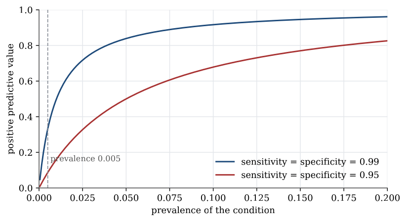
The threshold that defines a positive test trades sensitivity against specificity. A low threshold catches more cases and raises 1-\beta, and it also raises \alpha. A screening programme that must not miss a case sets the threshold so that the sensitivity is close to one, accepts a large \alpha, and applies a second, more specific test only to the positives. The PPV of the first test is then deliberately allowed to be modest. The PPV of the two-test sequence is the quantity that matters, and it is computed from the joint event “both tests positive”.
There is a reporting version of the same formula. Suppose a negative result is written up as a positive result with probability u, whether or not the condition is present, and a genuinely positive result is always reported. Then
\mathbb{P}(\text{reported positive}\mid D)=(1-\beta)+u\beta, \qquad \mathbb{P}(\text{reported positive}\mid D^c)=\alpha+u(1-\alpha),
and the PPV of a reported positive replaces 1-\beta and \alpha in the Bayes formula by those two mixtures. The bias u is not sampling noise. Sampling noise is already in \alpha and \beta. The bias is a systematic misreporting of the sign. Any u>0 moves false results into the reported-positive pile and lowers the PPV.
Repeating an independent test changes the odds in the other direction. If n independent tests must all be positive, and each has the same sensitivity and specificity, the likelihood ratio of that joint event is \{(1-\beta)/\alpha\}^n. The posterior odds are R times that ratio. Whenever 1-\beta>\alpha, the ratio exceeds one and the posterior odds tend to infinity with n, so the PPV of the joint positive result tends to 1. One significant result is a single factor (1-\beta)/\alpha. A procedure that rarely fails to repeat is a power of that factor. The PPV of an unreplicated result can stay low because R is low. The PPV of a result that survives several independent repetitions does not.
# PPV from prevalence, sensitivity and specificity.
ppv <- function(prevalence, sensitivity, specificity) {
  p1 <- prevalence
  alpha <- 1 - specificity
  beta <- 1 - sensitivity
  p1 * (1 - beta) / (p1 * (1 - beta) + (1 - p1) * alpha)
}
ppv(0.005, 0.95, 0.95)    # 0.0872
ppv(0.001 / 1.001, 0.99, 0.99)  # prior odds 0.001, about 0.090
Used in
- Taught in Predictive values of a test
- Questions that use it (2) — A rare condition · The matching negative predictive value (answer)
- All 2 questions on Predictive values of a test
See also
Negative predictive value · Fallacy of the transposed conditional · Sensitivity and specificity