Most powerful tests
Advanced
A test fixes a null hypothesis and a type I error, and then looks for the critical region with the smallest type II error. For two simple hypotheses the most powerful test rejects for a large likelihood ratio.
What you need first. Read Hypothesis tests.
Part of Statistical inference · 2 questions on this topic · What links here
Most powerful tests
| Part | Statistical inference |
| Level | Advanced |
| Chapter | 8 of 16 in this part |
| Previous | Hypothesis tests |
| Next | Generalised likelihood-ratio tests |
| Questions | 2 |
| Figures | 1 |
A test fixes a null hypothesis and asks for a critical region whose type I error stays at a chosen level, and whose type II error is as small as possible. For two simple hypotheses that region is given by the likelihood ratio. The result is the Neyman–Pearson lemma. When the alternative is one-sided and the likelihood ratio orders the sample the same way for every alternative, the same region is uniformly most powerful. A two-sided alternative does not have that property.
The definitions of size, power and the Neyman–Pearson approach are on the hypothesis-testing page. This page constructs the region.
Likelihood ratio for two simple hypotheses
Let the data be a sample x, and suppose the model is completely specified by one or the other of two values of the parameter. The hypotheses
H_0:\theta=\theta_0, \qquad H_1:\theta=\theta_1
are both simple. Write L(\theta;x) for the likelihood. If L(\theta_0;x)/L(\theta_1;x) is small, the observed sample is much more probable under \theta_1 than under \theta_0. The likelihood-ratio test rejects H_0 when
\frac{L(\theta_0;x)}{L(\theta_1;x)}\le c
for a threshold c chosen so that the type I error equals \alpha, or comes as close as a discrete statistic allows. Equivalently, the critical region is
R=\bigl\{x: L(\theta_1;x)/L(\theta_0;x)>k\bigr\},
the form used to prove the Neyman–Pearson lemma. The two descriptions differ only by taking a reciprocal and renaming the constant.
For a normal sample with known variance the ratio collapses to the sample mean. Let X_j be independent \operatorname{N}(\mu,\sigma^2) and test \mu=\mu_0 against \mu=\mu_1, with \mu_1>\mu_0. The log likelihood ratio is
\log\frac{L(\mu_1)}{L(\mu_0)}=-\frac{1}{2\sigma^2}\sum_j\bigl\{(X_j-\mu_1)^2-(X_j-\mu_0)^2\bigr\}=\frac{n}{\sigma^2}\Bigl\{\overline X(\mu_1-\mu_0)-\tfrac12(\mu_1^2-\mu_0^2)\Bigr\}.
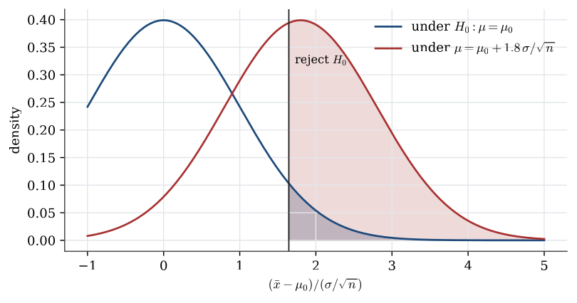
Because \mu_1-\mu_0>0, the ratio is large exactly when \overline X is large. The test rejects when \overline X>k. The threshold that has size \alpha comes from the null distribution \overline X\sim\operatorname{N}(\mu_0,\sigma^2/n):
\alpha=\mathbb{P}_{\mu_0}(\overline X>k)=\mathbb{P}\Bigl(Z>\frac{k-\mu_0}{\sigma/\sqrt n}\Bigr), \qquad k=\mu_0+z_{1-\alpha}\,\frac{\sigma}{\sqrt n},
where Z is standard normal and z_{1-\alpha}=\Phi^{-1}(1-\alpha). If instead \mu_1<\mu_0, the inequality reverses and the test rejects for small \overline X, with k=\mu_0-z_{1-\alpha}\,\sigma/\sqrt n.
The same reduction is why a known-variance z test was already the procedure on the hypothesis-testing page. The likelihood ratio says it is not merely a convenient pivot. For this pair of means it is the most powerful test of its size.
Neyman–Pearson lemma
Main article: Neyman–Pearson lemma
Among all tests of H_0:\theta=\theta_0 against H_1:\theta=\theta_1 with type I error at most \alpha, the likelihood-ratio test has the greatest power.
Let R be the likelihood-ratio region \{x:L(\theta_1;x)>k\,L(\theta_0;x)\}, with k chosen so that \int_R L(\theta_0;x)\,dx=\alpha. Let R^\star be any other region with the same size, \int_{R^\star} L(\theta_0)=\alpha. Write \pi(R)=\int_R L(\theta_1) for the power. Split each region into the part it shares and the part it does not:
\pi(R)-\pi(R^\star)=\int_{R\cap (R^\star)^c}L(\theta_1)-\int_{(R)^c\cap R^\star}L(\theta_1).
On R\cap(R^\star)^c the likelihood ratio exceeds k, and on (R)^c\cap R^\star it does not. Replacing L(\theta_1) by k\,L(\theta_0) therefore lowers the first integral and raises the second, and the difference is at least
k\int_{R\cap(R^\star)^c}L(\theta_0)-k\int_{(R)^c\cap R^\star}L(\theta_0)=k\int_R L(\theta_0)-k\int_{R^\star}L(\theta_0)=k\alpha-k\alpha=0.
Hence \pi(R)\ge\pi(R^\star). A discrete distribution may not hit \alpha exactly. The same argument applies to a randomised test that rejects with a fractional probability on the boundary point where the likelihood ratio equals k; without randomisation the most powerful test is the largest likelihood-ratio region whose size does not exceed \alpha. The binomial serve test on the hypothesis-testing page is that discrete case: at level 0.05 the region \{13,14,15\} has size 0.027, and the next larger region already has size 0.091.
The lemma compares two completely specified distributions. It does not by itself choose a test that is good for every alternative at once. That is the next definition.
Uniformly most powerful test
Main article: Uniformly most powerful test
Let the alternative be composite, H_1:\theta\in\Omega_1. A test is uniformly most powerful at level \alpha if its size is at most \alpha and, for every \theta_1\in\Omega_1, it is most powerful against the simple alternative \theta=\theta_1.
For a normal mean with known variance and H_1:\mu>\mu_0, pick any \mu_1>\mu_0. The Neyman–Pearson test of \mu_0 against that \mu_1 rejects for \overline X>k with the same k=\mu_0+z_{1-\alpha}\,\sigma/\sqrt n, whatever \mu_1 was. The critical region does not depend on which alternative was used to build the ratio. It is therefore most powerful against every \mu_1>\mu_0, and the one-sided z test is uniformly most powerful.
The power at a particular \mu_1 is
\mathbb{P}_{\mu_1}(\overline X>k)=\Phi\Bigl(-z_{1-\alpha}+\frac{\mu_1-\mu_0}{\sigma/\sqrt n}\Bigr).
It increases with (\mu_1-\mu_0)\sqrt n/\sigma. A test can be uniformly most powerful and still have poor power if n is small or \sigma is large. Uniformity is a comparison with other tests of the same size, not a promise that the power is high.
The one-sided Poisson test has the same structure. For X_j independent Poisson(\lambda) and H_0:\lambda=\lambda_0 against H_1:\lambda>\lambda_0, the likelihood ratio is large when \sum X_j is large, for every \lambda_1>\lambda_0. The uniformly most powerful test rejects when \sum X_j\ge d, with d the smallest integer whose null probability \mathbb{P}\{\operatorname{Poisson}(n\lambda_0)\ge d\} does not exceed \alpha.
A t test of the same mean, which replaces the Poisson variance by the sample variance, is a different procedure. When the data are Poisson the likelihood-ratio test has the higher power. When they are not, the Poisson test can have a type I error far from \alpha, while the t statistic still has an approximate t null distribution under a finite variance. The lemma’s optimality is inside the model used to write the likelihood. It does not survive an arbitrary change of that model. The large-sample comparison of the two procedures is on Large-sample estimation.
A rule that is not a function of a statistic chosen before seeing the data is not in this competition at all. Rejecting when one particular patient’s improvement exceeds a threshold picked after looking at who improved can have any type I error one wants to claim, because the region was fitted to the sample. The power calculation for the one-sided normal test starts from a region R that does not depend on which sample was drawn.
Uniformly most powerful unbiased test
Main article: Uniformly most powerful unbiased test
Now let H_1:\mu\ne\mu_0, still with known normal variance. Against an alternative \mu_1>\mu_0 the most powerful test rejects for large \overline X. Against \mu_1<\mu_0 it rejects for small \overline X. Those are different regions. No single region is most powerful against both. A uniformly most powerful test of the two-sided hypothesis does not exist.
The usual two-sided z test rejects when |\overline X-\mu_0|>z_{1-\alpha/2}\,\sigma/\sqrt n. It is not most powerful against a one-sided alternative: the one-sided test of the same size puts all of its critical probability on the side where that alternative lives, and therefore has higher power there. The two-sided test spends half its type I error on a side the one-sided alternative says cannot occur.
What the two-sided test does have is unbiasedness. A test is unbiased when its power is at least \alpha at every alternative. The one-sided test fails that requirement for the two-sided problem: against an alternative on the other side its power is less than \alpha. Among unbiased tests, the equal-tailed region is uniformly most powerful. It is the uniformly most powerful unbiased test of H_0:\mu=\mu_0 against H_1:\mu\ne\mu_0. The threshold is
k=z_{1-\alpha/2}\,\frac{\sigma}{\sqrt n},
and the critical region is |\overline X-\mu_0|>k.
The same split explains the t test when \sigma is unknown. Replacing \sigma by s in the likelihood ratio, using the joint normal likelihood of the sample, reduces a one-sided test to a one-sided t_{n-1} critical value and a two-sided test to the equal-tailed t critical value. The unknown variance is estimated by the residual sum of squares, which is independent of \overline X in a normal sample, and the ratio is the t pivot already used for confidence intervals. The duality is exact: the two-sided level-\alpha test accepts \mu_0 if and only if the level 1-\alpha interval contains \mu_0.
# Level 0.05 critical value for a two-sided t test, n = 42.
qt(0.975, df = 41)     # 2.020
# A one-sided test at the same level uses the 0.95 quantile, which is smaller.
qt(0.95, df = 41)      # 1.683
The one-sided quantile is smaller because the whole type I error sits in one tail. Using it for a two-sided scientific question, after seeing the sign of \overline X-\mu_0, is the one-sided test with a direction chosen from the data. Its type I error is then about 2\alpha, not \alpha.
For two simple hypotheses the most powerful test of a given size rejects when the likelihood under the alternative is large relative to the likelihood under the null. If every alternative in a one-sided family produces the same region, the test is uniformly most powerful. A two-sided normal mean has no such test. The equal-tailed test is the most powerful test inside the smaller class of unbiased tests.
Questions on this topic
Open a question to attempt it. Its worked answer is folded away at the bottom of the page.
2 questions.
| Question | Level | Answer |
|---|---|---|
| A critical value from the lemma | Advanced | ✓ |
| Why the two-sided test is not UMP | Advanced | ✓ |
What links here
Pages (5)
- Statistical inference — via most powerful
- Information and bounds — via Most powerful tests
- Hypothesis tests — via Neyman–Pearson lemma
- Generalised likelihood-ratio tests — via Most powerful tests, Neyman–Pearson lemma
- Testing examples — via Neyman–Pearson lemma
Questions and answers (1)