One-factor analysis of variance
Section of Analysis of variance, part of Statistical inference · Also in Analysis of variance examples
One-factor analysis of variance
| Type | Section |
| Taught in | Analysis of variance · Analysis of variance examples |
| Part | Statistical inference · Data analysis |
| Questions using it | 2 |
In Analysis of variance
From Analysis of variance
Definition 1 (One-way analysis of variance) In a completely randomised one-factor design, responses at level j=1,\ldots,k follow
Y_{ij}=\mu_j+\varepsilon_{ij}, \qquad \varepsilon_{ij}\ \text{independent}\ \operatorname{N}(0,\sigma^2),
with n_j observations at level j and n=\sum_j n_j. The levels are the treatments. The hypothesis of equal means is H_0:\mu_1=\cdots=\mu_k.
The model is the k-sample version of the two-sample t model: k independent normal samples with a common variance. \mu_j is the true mean at level j, and \varepsilon_{ij} is the deviation of observation i from it. The model has k+1 unknown parameters. Write \overline Y_{\cdot j} for the mean at level j and \overline Y_{\cdot\cdot} for the grand mean of all n observations. The maximum likelihood estimators are
\widehat\mu_j=\overline Y_{\cdot j},\qquad \widehat\sigma^2=\frac1n\sum_{j=1}^k\sum_{i=1}^{n_j}(Y_{ij}-\overline Y_{\cdot j})^2,
by the same calculation as for one normal sample, done group by group with a shared variance. For the heart rates, \widehat\sigma^2=935.5/40=23.4.
Proposition 1 (ANOVA sum of squares decomposition) With
\mathrm{SS}_{\mathrm{total}}=\sum_{j=1}^k\sum_{i=1}^{n_j}(Y_{ij}-\overline Y_{\cdot\cdot})^2, \qquad \mathrm{SS}_{\mathrm{treatment}}=\sum_{j=1}^k n_j(\overline Y_{\cdot j}-\overline Y_{\cdot\cdot})^2, \qquad \mathrm{SS}_{\mathrm{error}}=\sum_{j=1}^k\sum_{i=1}^{n_j}(Y_{ij}-\overline Y_{\cdot j})^2,
the total sum of squares splits as \mathrm{SS}_{\mathrm{total}}=\mathrm{SS}_{\mathrm{treatment}}+\mathrm{SS}_{\mathrm{error}}.
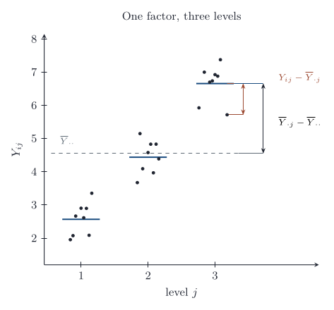
Write each deviation from the grand mean as a deviation of the group mean plus a deviation within the group, Y_{ij}-\overline Y_{\cdot\cdot}=(\overline Y_{\cdot j}-\overline Y_{\cdot\cdot})+(Y_{ij}-\overline Y_{\cdot j}), and square. The cross term vanishes group by group,
\sum_{j=1}^k(\overline Y_{\cdot j}-\overline Y_{\cdot\cdot})\sum_{i=1}^{n_j}(Y_{ij}-\overline Y_{\cdot j})=0,
because deviations from a group mean sum to zero within that group. \mathrm{SS}_{\mathrm{treatment}} measures variation between the groups and \mathrm{SS}_{\mathrm{error}} measures variation within them.
Theorem 1 (ANOVA F distribution) In the one-way model, \mathrm{SS}_{\mathrm{error}}/\sigma^2 is \chi^2_{n-k}, and it is independent of \mathrm{SS}_{\mathrm{treatment}}. Under H_0:\mu_1=\cdots=\mu_k, \mathrm{SS}_{\mathrm{treatment}}/\sigma^2 is \chi^2_{k-1}, and therefore
F=\frac{\mathrm{SS}_{\mathrm{treatment}}/(k-1)}{\mathrm{SS}_{\mathrm{error}}/(n-k)}=\frac{\mathrm{MS}_{\mathrm{treatment}}}{\mathrm{MS}_{\mathrm{error}}}
has the F_{k-1,\,n-k} distribution.
Each group is a normal sample, so by the normal sample theorem its within-group sum of squares over \sigma^2 is \chi^2_{n_j-1}, independent of its own mean. The groups are independent, so the within-group sums are independent of one another and of all the group means. Adding them, \mathrm{SS}_{\mathrm{error}}/\sigma^2 is \chi^2_{n-k}, since \sum(n_j-1)=n-k. \mathrm{SS}_{\mathrm{treatment}} is a function of the group means alone, so it is independent of \mathrm{SS}_{\mathrm{error}}. Under H_0, set W_j=\sqrt{n_j}(\overline Y_{\cdot j}-\mu)/\sigma; these are independent standard normals, and \mathrm{SS}_{\mathrm{treatment}}/\sigma^2 is the squared length of the vector {\boldsymbol{W}} after its component along (\sqrt{n_1},\ldots,\sqrt{n_k}) is removed. That leaves k-1 dimensions, and the rotation argument of the normal sample theorem gives \chi^2_{k-1}. The ratio of the two, each divided by its degrees of freedom, is F_{k-1,n-k} by definition.
The mean squares \mathrm{MS}=\mathrm{SS}/\text{degrees of freedom} are estimates of \sigma^2. \mathrm{MS}_{\mathrm{error}} estimates it whatever the means. \mathrm{MS}_{\mathrm{treatment}} estimates it only under H_0; if the means differ, its expectation is larger. The level-\alpha test therefore rejects for large F, when F\ge F_{k-1,\,n-k;\,1-\alpha}. The calculations are set out in an analysis-of-variance table.
| Source | Degrees of freedom | Sum of squares | Mean square | F |
|---|---|---|---|---|
| Treatment | k-1 | \mathrm{SS}_{\mathrm{treatment}} | \mathrm{MS}_{\mathrm{treatment}} | \mathrm{MS}_{\mathrm{treatment}}/\mathrm{MS}_{\mathrm{error}} |
| Error | n-k | \mathrm{SS}_{\mathrm{error}} | \mathrm{MS}_{\mathrm{error}} | |
| Total | n-1 | \mathrm{SS}_{\mathrm{total}} |
For the heart rates, \mathrm{SS}_{\mathrm{treatment}}=67.475 on 3 degrees of freedom and \mathrm{SS}_{\mathrm{error}}=935.500 on 36, so F=22.49/25.99=0.866, against F_{3,36;0.95}=2.87. The p-value is 0.47. The age groups show no difference in mean increase.
With k=2 this F equals the square of the pooled two-sample t statistic, and the test is the same test.
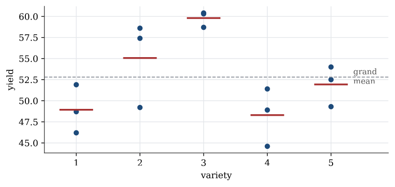
Example 1 (Five varieties of corn) Five varieties of corn are each grown on three plots.
| Variety | 1 | 2 | 3 | 4 | 5 |
|---|---|---|---|---|---|
| Yields | 46.2, 51.9, 48.7 | 49.2, 58.6, 57.4 | 60.3, 58.7, 60.4 | 48.9, 51.4, 44.6 | 52.5, 54.0, 49.3 |
| Mean | 48.93 | 55.07 | 59.80 | 48.30 | 51.93 |
Question. Do the varieties differ in mean yield?
Solution. The grand mean is 52.81. Then \mathrm{SS}_{\mathrm{treatment}}=3\sum_j(\overline y_{\cdot j}-52.81)^2=270.3 on 4 degrees of freedom, and \mathrm{SS}_{\mathrm{error}}=105.7 on 10.
| Source | Df | SS | MS | F | p |
|---|---|---|---|---|---|
| Variety | 4 | 270.3 | 67.57 | 6.39 | 0.008 |
| Error | 10 | 105.7 | 10.57 | ||
| Total | 14 | 375.9 |
The p-value is 0.008, so the varieties differ. The pooled standard deviation is \sqrt{10.57}=3.25. The F test says only that the five means are not all equal; which varieties differ is the next question.
Contrasts
Main article: Contrast
Definition 2 (Contrast) A contrast is a linear combination C=\sum_j c_j\mu_j of the treatment means whose coefficients sum to zero. It is estimated by \widehat C=\sum_j c_j\overline Y_{\cdot j}, which is unbiased with variance \sigma^2\sum_j c_j^2/n_j.
A contrast tests a sub-hypothesis that was formulated before the data were seen. With \mathrm{SS}_C=\widehat C^2/\sum_jc_j^2/n_j, under H_0:C=0 the ratio \mathrm{SS}_C/\sigma^2 is \chi^2_1, independent of \mathrm{SS}_{\mathrm{error}}, so
F=\frac{\mathrm{SS}_C}{\mathrm{MS}_{\mathrm{error}}}
has the F_{1,\,n-k} distribution. The first part holds because \widehat C is normal with mean 0 under H_0, and \mathrm{SS}_C/\sigma^2 is its square over its variance. Contrasts that were chosen because the data suggested them do not keep that null distribution. A contrast has to be chosen from the scientific question, not from the ranking of the observed means.
Suppose varieties 1, 2, 4 and 5 of corn are mutations of one parent strain and variety 3 is not, so the question is whether variety 3 differs from the average of the others. The contrast is C=(\mu_1+\mu_2+\mu_4+\mu_5)/4-\mu_3, with estimate
\widehat C=\frac{48.93+55.07+48.30+51.93}{4}-59.80=-8.74,
and \sum c_j^2/n_j=(4/16+1)/3=0.4167. So F=(-8.74)^2/0.4167/10.57=17.4 on (1,10) degrees of freedom, with p-value 0.002. Variety 3 yields more than the mutant average.
Multiple comparisons
Main article: Multiple comparisons
Comparing every pair of means with its own 95% interval inflates the chance that some interval misses. With five varieties there are ten pairs, and the chance that at least one of ten 95% intervals misses can be far above 5%. Tukey’s intervals control that simultaneous error.
Definition 3 (Tukey intervals) In a one-way design with k groups of equal size r, and n=kr, the probability is 1-\alpha that every one of the \binom k2 differences \mu_i-\mu_j simultaneously satisfies
\overline Y_{\cdot i}-\overline Y_{\cdot j}-D\sqrt{\mathrm{MS}_{\mathrm{error}}}<\mu_i-\mu_j<\overline Y_{\cdot i}-\overline Y_{\cdot j}+D\sqrt{\mathrm{MS}_{\mathrm{error}}}, \qquad D=\frac{Q_{k,\,n-k;\,1-\alpha}}{\sqrt r},
where Q_{k,\,n-k;\,1-\alpha} is the quantile of the studentised range for k groups and n-k error degrees of freedom.
The studentised range is the law of the largest minus the smallest of k independent standard normals, divided by an independent \sqrt{V/m} with V\sim\chi^2_m. Bounding the largest difference among the group means bounds all of them at once. A pair whose interval excludes zero is declared different at familywise level \alpha.
For the corn, k=5, r=3 and n-k=10, so Q_{5,10;0.95}=4.654 and the half-width of every interval is 4.654\sqrt{10.57/3}=8.74. The ten intervals for \mu_i-\mu_j are
| j=2 | j=3 | j=4 | j=5 | |
|---|---|---|---|---|
| i=1 | (-14.87,\ 2.60) | (-19.60,\ -2.13) | (-8.10,\ 9.37) | (-11.74,\ 5.74) |
| i=2 | (-13.47,\ 4.00) | (-1.97,\ 15.50) | (-5.60,\ 11.87) | |
| i=3 | (2.76,\ 20.24) | (-0.87,\ 16.60) | ||
| i=4 | (-12.37,\ 5.10) |
Two exclude zero: variety 3 yields more than variety 1 and more than variety 4. No other pair can be separated at familywise level 0.05.
In Analysis of variance examples
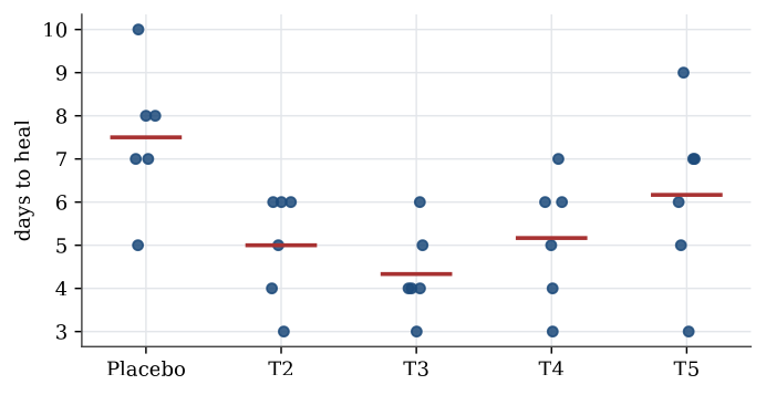
Example 2 (Five treatments for cold sores) Thirty patients with cold sores were assigned at random to five treatments, six to each; treatment 1 is a placebo. The days until the sore healed were
| Placebo | T2 | T3 | T4 | T5 |
|---|---|---|---|---|
| 5 | 4 | 6 | 7 | 9 |
| 8 | 6 | 4 | 4 | 3 |
| 7 | 6 | 4 | 6 | 5 |
| 7 | 3 | 5 | 6 | 7 |
| 10 | 5 | 4 | 3 | 7 |
| 8 | 6 | 3 | 5 | 6 |
Question. Do the treatments differ in mean healing time?
Solution. The table is not in standard form: for an analysis the healing times must be one column and the treatment a factor in another. stack does that.
x <- data.frame(Placebo = c(5, 8, 7, 7, 10, 8), T2 = c(4, 6, 6, 3, 5, 6),
                T3 = c(6, 4, 4, 5, 4, 3), T4 = c(7, 4, 6, 6, 3, 5),
                T5 = c(9, 3, 5, 7, 7, 6))
coldsore <- stack(x)
names(coldsore) <- c("times", "treatment")
tapply(coldsore$times, coldsore$treatment, mean)
# Placebo  T2    T3    T4    T5
#   7.500 5.000 4.333 5.167 6.167
coldsore.lm <- lm(times ~ treatment, data = coldsore)
anova(coldsore.lm)
#           Df Sum Sq Mean Sq F value  Pr(>F)
# treatment  4 36.467  9.1167  3.896 0.01359
# Residuals 25 58.500  2.3400
Under equal means F=3.90 would come from an F_{4,25} distribution, and the p-value is 0.014, so the treatments do differ. The placebo has the longest mean healing time, 7.5 days. The residual mean square, 2.34, estimates the common variance, so the within-group standard deviation is about 1.5 days.
Checking the model
Main article: Checking an analysis-of-variance model
The F test assumes independent normal errors with the same variance in every group. These are checked through the residuals, y_{ik}-\overline y_{i\cdot}: a plot of residuals against fitted values should show no pattern and similar spread in each group, and a normal quantile plot of the residuals should be close to a straight line.
plot(coldsore.lm, 1:2) # residuals against fitted values, and a normal Q-Q plotIndependence is not something a residual plot can verify. It comes from the design: here, from assigning treatments to separate patients at random.
Which groups differ?
Main article: Which groups differ?
A significant F says the means are not all equal; it does not say which ones differ. Comparing every pair with its own test at level \alpha inflates the chance of a false difference, since with five groups there are ten pairs.
Definition 4 (Bonferroni correction) To make m comparisons with a familywise error rate of at most \alpha, run each at level \alpha/m. Equivalently, multiply each p-value by m, capping at 1.
The correction works because the probability that at least one of m events occurs is at most the sum of their probabilities. It is simple and always valid, but conservative when m is large. Tukey intervals, built for all pairwise differences of means, are sharper. For the cold sores, Tukey’s method at familywise level 0.05 separates only one pair: placebo against treatment 3, with difference 3.17 days and 95% simultaneous interval (0.57,\ 5.76). The Bonferroni version agrees: the t statistic for that pair is 3.59, beyond the corrected critical value t_{25;\,1-0.05/20}=3.08, and no other pair passes.
TukeyHSD(aov(times ~ treatment, data = coldsore))
pairwise.t.test(coldsore$times, coldsore$treatment, p.adjust.method = "bonferroni")
The same question arises with unequal groups. Haemoglobin was measured for three forms of sickle-cell disease, in groups of 16 (HbSS), 15 (HbST) and 10 (HbSC). The analysis of variance gives a treatment sum of squares of 99.89 on 2 degrees of freedom and an error mean square of 1.00 on 38, so F=49.9 and the p-value is about 2.3\times10^{-11}. Bonferroni-corrected pairwise tests, with three comparisons each at level 0.05/3, then say which forms differ; the exercises work through them.
Used in
- Taught in Analysis of variance · Analysis of variance examples
- Also used in Analysis of variance examples · Linear model examples
- Questions that use it (2) — Two groups · Haemoglobin and sickle-cell type
- All 6 questions on Analysis of variance
See also
One-way analysis of variance · ANOVA sum of squares decomposition · ANOVA F distribution · Contrast · Tukey intervals · Randomised block design · Between and within · Multiple comparisons