Sleep-deprivation data
Section of Random slopes, and a binary mixed model, part of Correlated data
Sleep-deprivation data
| Type | Section |
| Taught in | Random slopes, and a binary mixed model |
| Part | Correlated data |
Eighteen subjects, treated as a sample of long-distance drivers rather than as eighteen named people, were restricted to three hours of sleep a night for ten days. Each day their reaction time was an average of several ruler-drop trials, in milliseconds. Most people slow down. One or two stay flat, and one seems to get slightly faster, which is the pattern if three hours was more sleep than they usually had. Before looking, the reasonable model is a person-specific intercept and a person-specific slope on day. Reflexes differ, and so does the damage from another night of three hours.
need <- function(pkg) {
  if (!requireNamespace(pkg, quietly = TRUE)) {
    install.packages(pkg, repos = "https://cloud.r-project.org")
  }
  suppressPackageStartupMessages(library(pkg, character.only = TRUE))
}
need("lme4")
data(sleepstudy, package = "lme4")
fit <- lmer(Reaction ~ Days + (Days | Subject), data = sleepstudy)
summary(fit)
fit0 <- lmer(Reaction ~ Days + (1 | Subject), data = sleepstudy)
anova(fit0, fit)
round(ranef(fit)$Subject[c("308", "309", "370"), ], 1)
The (Days | Subject) term is a random intercept and a random slope on day, with a correlation between them. The fit is by restricted maximum likelihood. The estimates are
Random effects:
 Subject  (Intercept)   variance 612.09    sd 24.74
          Days          variance  35.07    sd  5.92    corr 0.07
 Residual               variance 654.94    sd 25.59

Fixed effects:
 (Intercept)   251.41     se 6.83
 Days           10.47     se 1.55
These are statements about the population the eighteen were drawn from, not about the eighteen. The average driver starts at 251 milliseconds and slows by 10.5 milliseconds per day of deprivation. A typical driver sits 25 milliseconds away from that starting value, and a typical slope sits 5.9 milliseconds per day away from 10.5. The correlation between a driver’s intercept and slope is 0.07. Someone who is slow on day zero is not, in any important way, someone who deteriorates faster.
Whether the random slopes are needed is a comparison of this fit with Reaction ~ Days + (1 | Subject). The likelihood-ratio statistic is 42.1 on 2 degrees of freedom, and the printed p-value is 7\times 10^{-10}. That p-value is not an exact chi-squared tail probability. The null hypothesis puts a variance on the boundary of the parameter space, at zero, so the usual asymptotic distribution does not apply. The printed tail probability is conservative: it is larger than the p-value from the correct mixture of chi-squared laws. A conservative p-value this small is still small. The slopes stay. Had the printed value been 0.07, it would not be clear which side of 0.05 the proper test sat on, and the term would not be dropped on the strength of the printed value.
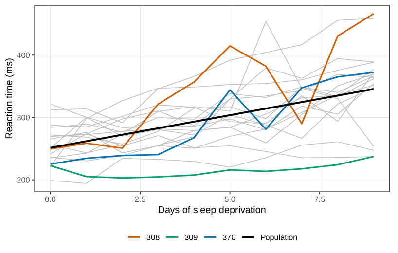
The empirical predictors of the eighteen deviations are a different object again. Subject 308 is predicted about 2 milliseconds slower than the population intercept and about 9 milliseconds per day steeper than the population slope. Subject 309 is about 40 milliseconds faster at the start and has a slope about 8 below the average, which is why that series looks flat: 10.5-8 is nearly zero. Subject 370 starts faster than average and then falls away faster than average.
Repeat the study and none of these eighteen numbers returns. The fixed effects 251 and 10.5 are the quantities that are supposed to.