Generalised linear mixed model

Section of Random slopes, and a binary mixed model, part of Correlated data

Type	Section
Taught in	Random slopes, and a binary mixed model
Part	Correlated data
Questions using it	3

The outer distribution does not have to be normal. Keep the linear predictor, random intercept and random slopes included, and let Y_{ji}\mid {\boldsymbol{X}}_{ji},\boldsymbol{\alpha}_j \stackrel{\mathrm{ind}}{\sim} \mathrm{Bernoulli}\!\left( \mu\bigl({\boldsymbol{X}}_{ji}^\top\boldsymbol{\beta}+{\boldsymbol{Z}}_{ji}^\top\boldsymbol{\alpha}_j\bigr) \right), with \boldsymbol{\alpha}_j still multivariate normal on the link scale. For a logit, \mu is the expit. The normal distribution on \boldsymbol{\alpha}_j is a modelling choice about a latent intercept, not a claim that we observed a normal measurement. It is a distribution we can interpret, and there is no stronger reason, before seeing the data, to pick a different one. The likelihood integrates the random effects out. There is no closed form, and no single algorithm that is guaranteed to find the maximum in every data set. When the numerical answer is in doubt, we fit the model more than one way, and we trust an agreement.

The 1989 Bangladesh fertility survey has 1934 women and a binary response: currently using contraception, or not. Age is centred and enters as a quadratic, because use should rise and then fall rather than climb forever. ch records whether she already has a living child. urban records urban against rural. district is the cluster. Women in the same district share facilities and customs, so a district intercept is the natural random effect. If every district in the country were in the sample, “a draw from a population of districts” would be a fiction about the boundaries of districts rather than about a sampling frame. We still use it. The districts that exist are one way of cutting the map.

need <- function(pkg) {
  if (!requireNamespace(pkg, quietly = TRUE)) {
    install.packages(pkg, repos = "https://cloud.r-project.org")
  }
  suppressPackageStartupMessages(library(pkg, character.only = TRUE))
}
need("lme4")
need("mlmRev")
data(Contraception, package = "mlmRev")
# age is already centred in this copy of the survey
Contraception$ch <- as.integer(Contraception$livch != "0")
Contraception$age2 <- Contraception$age^2
# a warning about rescaling age and age2 can appear; the estimates are the table below
summary(glmer(use ~ age + age2 + urban + ch + (1 | district),
              data = Contraception, family = binomial))

There are 60 districts. The district intercept has estimated standard deviation 0.474 on the log-odds scale: from district to district, at a fixed age, urban status, and child status, the log-odds of use move by about half a unit. The fixed effects are

(Intercept)  -1.006    se 0.169    z -5.95
age           0.0063   se 0.0079   z  0.79
age2         -0.00464  se 0.00072  z -6.43
urbanY        0.693    se 0.121    z  5.74
ch            0.860    se 0.148    z  5.80

Age has a positive linear term that is not itself significant and a negative square that is. Together they are the upside-down parabola.

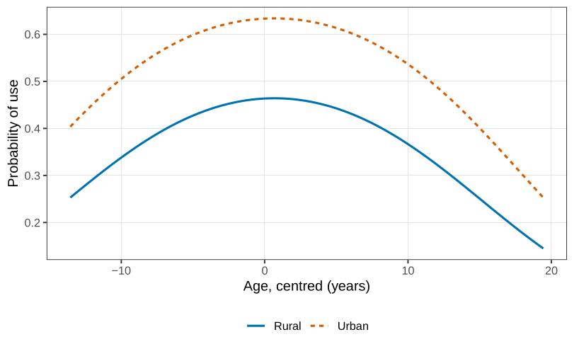
Figure 1: Fitted probability of contraceptive use against centred age, in a typical district, for a woman who already has a living child. Urban sits above rural. The two curves are one parabola, not two separate age effects.

The linear coefficient is not interpreted on its own. Urban women have odds of use \exp(0.693)=2.00 times those of rural women in the same district, at the same age and the same child status. A woman who already has a living child has odds \exp(0.860)=2.36 times those of a woman who does not. The district standard deviation is a typical shift, not a comparison of two named districts.

The urban contrast need not be the same in every district. A large city can have a rural fringe that is not very different from the centre. A small regional centre can have a sharp drop just outside the town. Some districts in the file are entirely urban, so a rural contrast for them is a prediction about a place that is not there.

need <- function(pkg) {
  if (!requireNamespace(pkg, quietly = TRUE)) {
    install.packages(pkg, repos = "https://cloud.r-project.org")
  }
  suppressPackageStartupMessages(library(pkg, character.only = TRUE))
}
need("lme4")
need("mlmRev")
data(Contraception, package = "mlmRev")
Contraception$ch <- as.integer(Contraception$livch != "0")
Contraception$age2 <- Contraception$age^2
summary(glmer(use ~ age + age2 + urban + ch + (urban | district),
              data = Contraception, family = binomial))

The average urban coefficient is now 0.770 (z=4.69): across districts, urban versus rural is a factor of \exp(0.77)\approx 2.16 on the odds. The district-level standard deviation of that contrast is 0.74, almost as large as the average contrast itself. Some districts have essentially no urban gap. Some have a much larger one. The correlation between the district intercept and the district urban slope is -0.79. A district that already has high use has a smaller urban-rural gap. Where use is common, rural and urban are not far apart, and where use is uncommon the town centre and the countryside are. The likelihood-ratio comparison with the random-intercept-only model is small enough, even as a conservative boundary p-value, that the extra random slope stays. It is an interaction. The effect of living in town depends on the district.

Marginal models, which describe the population average without a mechanism for the correlation, are the next chapter.

The sleep-study random-slope variance is 35.07. Convert it to a standard deviation and say what “a typical driver” means for the daily change in reaction time.
Why is the p-value on \sigma^2_{\text{slope}}=0 not a chi-squared tail probability, and in which direction is the printed value wrong?
From the contraception fit with a random intercept only, compute \exp(0.693) and \exp(0.860) and state both as odds ratios with the covariates that are being held fixed.
The correlation between a district’s intercept and its urban slope is -0.79. Give the direction of that statement in one sentence, without using the word “significant”.

Used in

Taught in Random slopes, and a binary mixed model
Questions that use it (3) — Toenail infection GLMM · Random intercepts and slopes · Conditional versus marginal effects
All 6 questions on Random slopes, and a binary mixed model

Used in

See also