Accidental-deaths data

Section of Forecasting, part of Time series

Type	Section
Taught in	Forecasting
Part	Time series

USAccDeaths is a monthly count of accidental deaths in the United States, six years, 72 months, ending in December 1978.

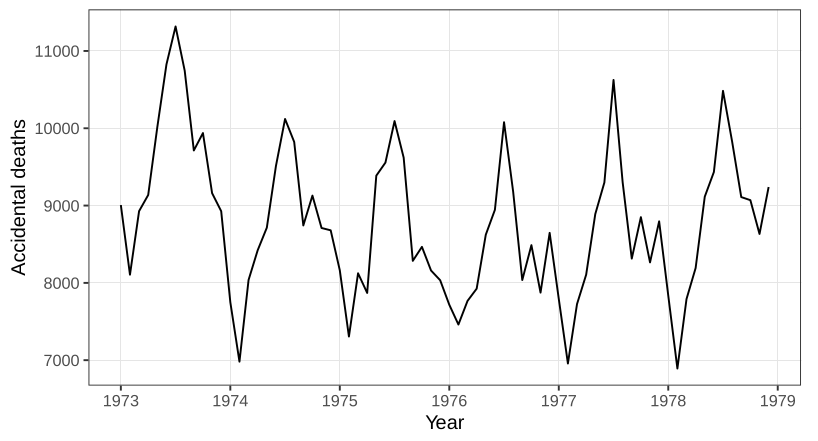
Figure 1: Monthly accidental deaths in the United States, 1973 to 1978. The series is not white noise: deaths are higher in the northern summer, and the level sags and then recovers.

Plotting a series that R already knows is a time series puts time on the horizontal axis. Figure is not white noise. Deaths are higher in the middle of the year, the northern summer, and lower in winter. A twelve-month cycle is the obvious feature. The overall level is not a straight trend. It sags and then recovers, the sort of slow movement produced when a temporary legal or behavioural change pulls a series down and then lets it drift back.

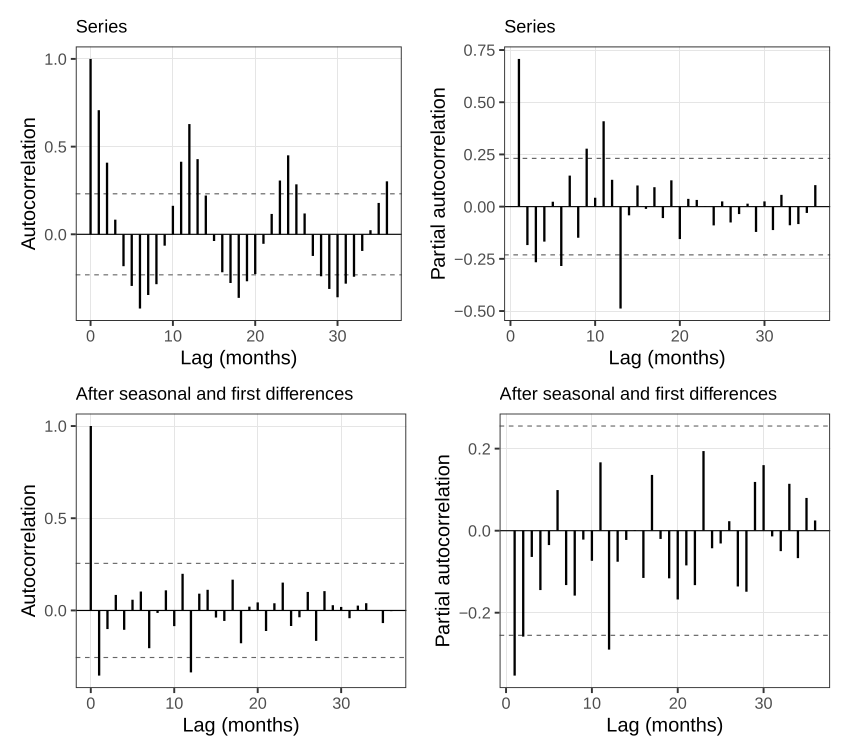
The autocorrelation and the partial autocorrelation both keep oscillating. An MA process would cut the autocorrelation off after a finite lag. An AR process would cut the partial autocorrelation off. Neither plot dies. That is the seasonality, still in the correlations.

Differencing at lag 12, \nabla_{12} X_t=X_t-X_{t-12}, removes a twelve-month cycle and, as a side effect, a linear trend. The differenced series still slopes. A linear trend left after a seasonal difference means the original series had a quadratic trend. One further difference at lag 1 takes that slope out. What remains is closer to a constant mean and a constant scatter. The autocorrelation of that twice-differenced series still has a spike at the first lag, and a spike near one year. Those are the MA terms.

Figure 2: Autocorrelation and partial autocorrelation, in months. The top row is the raw series: neither plot dies, and the year shows up at lags 12 and 24. The bottom row is the series after a seasonal difference and a first difference. What remains is a spike at lag 1 and a spike near lag 12.

auto.arima, with the seasonal option left on, finds this without being told that the data are monthly.

need <- function(pkg) {
  if (!requireNamespace(pkg, quietly = TRUE)) {
    install.packages(pkg, repos = "https://cloud.r-project.org")
  }
  suppressPackageStartupMessages(library(pkg, character.only = TRUE))
}
need("forecast")
fit <- auto.arima(USAccDeaths, seasonal = TRUE)
fit
fc <- forecast(fit, h = 12)
fc$mean[1]
sum(fc$mean)

The selected model differences once at lag 12, keeps a seasonal MA(1) on that yearly lag, differences once more at lag 1, and keeps an ordinary MA(1). There is no AR term. Both MA coefficients are negative. They are read as behaviour rather than as algebra. If last month was worse than the month before, this month is more careful, and the coefficient on that surprise is negative. If last year was worse than the year before, this year is more careful, and the seasonal coefficient is negative too. A good year, by the same arithmetic, is followed by a slack one. The AIC is what the function used to choose the orders. BIC is available and was not the default.

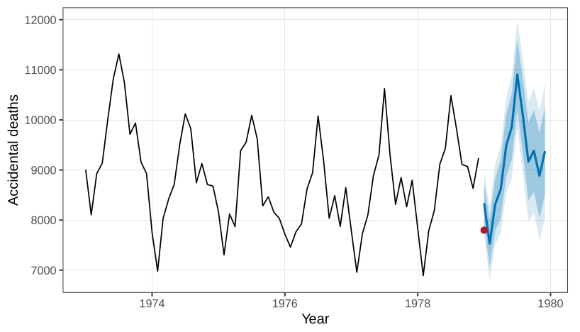
Figure 3: The forecast from January 1979. The darker band is the 80% interval and the lighter band is the 95% interval. The red point is the reported January total, 7798, inside the wider band and below the point forecast.

The series stops in December 1978. One step ahead, January 1979, the point forecast is 8336 deaths, with an 80% interval and a wider 95% interval. Figure is that forecast. The same step, read more roughly, is about 8400. The two figures are the same forecast read at two moments. The reported January total is 7798, inside the 95% band and low relative to the point forecast. Twelve steps ahead, the forecasts trace one more seasonal shape, and the sum of those twelve monthly forecasts was about 109{,}000. A reported annual total for 1979 is near 105{,}000. Further out, past a few years, the local MA terms die and the forecast repeats the seasonal shape on top of the quadratic trend. A long-range forecast from this model is the mean structure. A short-range forecast still feels the last surprise.

The function was not told the period. It found 12. That is the part worth trusting the automation for: it matched the differencing the seasonal plot would have suggested.

Used in

Taught in Forecasting
All 2 questions on Forecasting

Used in

See also