Traffic data

Section of Forecasting, part of Time series

Traffic data

Type	Section
Taught in	Forecasting
Part	Time series

WWWusage counts hits on a server, one number per minute for 100 minutes. There is no season in a series that short.

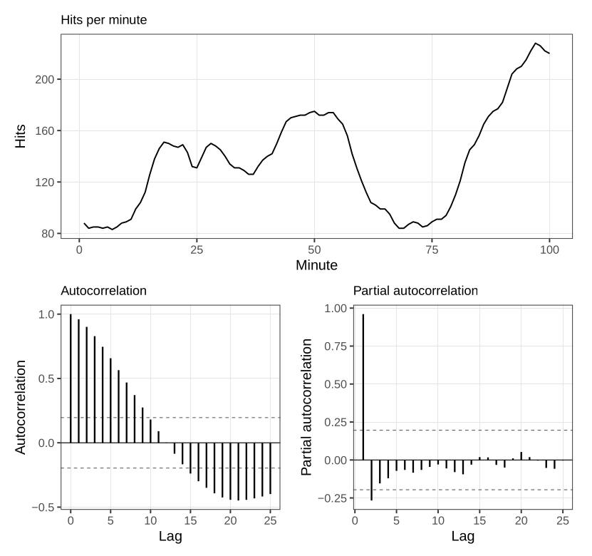
Figure 1: Server hits, one number per minute. The autocorrelation dies slowly and then changes sign, because the series wanders. The partial autocorrelation is essentially one spike, at lag 1.

The autocorrelation in Figure dies slowly. The partial autocorrelation dies after a lag or two. After one ordinary difference the series is closer to a flat mean, and auto.arima selects an ARMA(1,1) on that difference:

need <- function(pkg) {
  if (!requireNamespace(pkg, quietly = TRUE)) {
    install.packages(pkg, repos = "https://cloud.r-project.org")
  }
  suppressPackageStartupMessages(library(pkg, character.only = TRUE))
}
need("forecast")
auto.arima(WWWusage, seasonal = TRUE)

The fit has no seasonal piece: one difference, one autoregressive coefficient, and one moving-average coefficient. Both coefficients are positive. A busy minute is followed by a busy minute, and a minute that was busy relative to the minute before it is followed by a minute that is busier still. That is a trend, of the sort a topic has when it is spreading, and it does not need a separate time covariate.

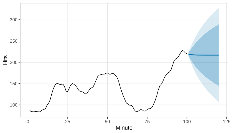
Figure 2: A twenty-minute forecast for the server traffic. The point forecast is nearly flat. The interval widens as the horizon moves away.

The forecast of the next minutes, in Figure, is a shallow line, and the interval widens as the horizon moves away. At a long horizon the forecast has forgotten the local level and sits on the mean that the difference implies.

Used in

Taught in Forecasting
All 2 questions on Forecasting

Used in

See also