Blocks in analysis of variance
Section of Analysis of variance, part of Statistical inference
Blocks in analysis of variance
| Type | Section |
| Taught in | Analysis of variance |
| Part | Statistical inference |
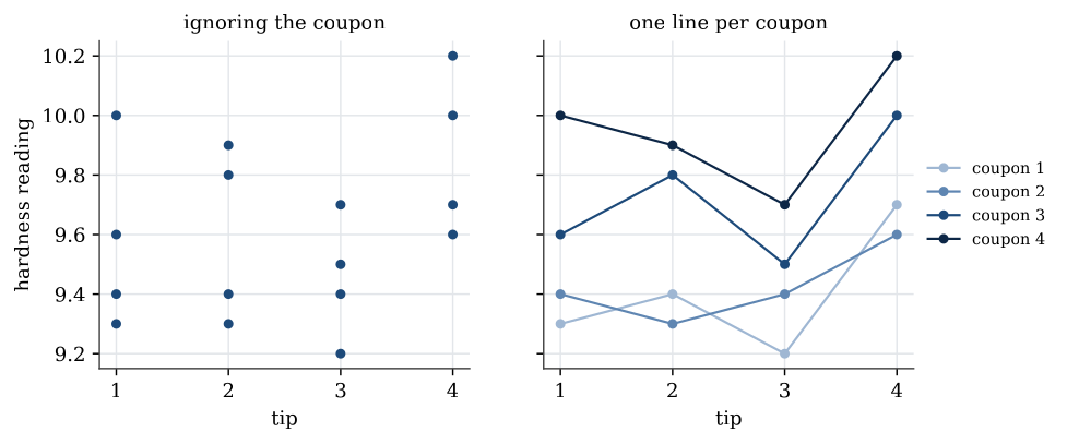
The hardness of a metal is measured by pressing a tester’s tip into a coupon of the metal. Four tips are each tested once on each of four coupons.
| Tip 1 | Tip 2 | Tip 3 | Tip 4 | |
|---|---|---|---|---|
| Coupon 1 | 9.3 | 9.4 | 9.2 | 9.7 |
| Coupon 2 | 9.4 | 9.3 | 9.4 | 9.6 |
| Coupon 3 | 9.6 | 9.8 | 9.5 | 10.0 |
| Coupon 4 | 10.0 | 9.9 | 9.7 | 10.2 |
Is there any difference between the tips? A one-way analysis with tip as the factor gives \mathrm{SS}_{\mathrm{tip}}=0.385 on 3 degrees of freedom and \mathrm{SS}_{\mathrm{error}}=0.905 on 12, so F=1.70 and p=0.22. No evidence of a difference.
But look at the coupons. Coupon 4 reads higher than coupon 1 under every tip. Much of the within-tip scatter is variation between coupons, and the one-way analysis lumps it into the error. Within each coupon, tip 4 reads highest and tip 3 lowest, almost every time.
Definition 1 (Randomised block design) A randomised block design measures every one of t treatments once in each of b blocks. The response for block i and treatment j is
Y_{ij}=\mu+\beta_i+\tau_j+\varepsilon_{ij}, \qquad \sum_{i=1}^b\beta_i=0,\quad\sum_{j=1}^t\tau_j=0,
with \varepsilon_{ij} independent and \operatorname{N}(0,\sigma^2). Here \mu is the overall mean, \beta_i the effect of block i and \tau_j the effect of treatment j.
Here the block effects \beta_i are fixed constants, one for each coupon in this study. When the blocks are themselves a sample from a larger population, such as hospitals, patients or fields, the block effects can instead be drawn from a distribution, which is the random intercept model.
The design is balanced: every block–treatment cell has the same number of observations, here one. The sums of squares are
\mathrm{SS}_{\mathrm{blocks}}=t\sum_{i=1}^b(\overline Y_{i\cdot}-\overline Y_{\cdot\cdot})^2, \qquad \mathrm{SS}_{\mathrm{treatment}}=b\sum_{j=1}^t(\overline Y_{\cdot j}-\overline Y_{\cdot\cdot})^2,
\mathrm{SS}_{\mathrm{error}}=\sum_{i=1}^b\sum_{j=1}^t(Y_{ij}-\overline Y_{i\cdot}-\overline Y_{\cdot j}+\overline Y_{\cdot\cdot})^2,
and the total splits as \mathrm{SS}_{\mathrm{total}}=\mathrm{SS}_{\mathrm{treatment}}+\mathrm{SS}_{\mathrm{blocks}}+\mathrm{SS}_{\mathrm{error}}, by the same cross-term argument as before. \mathrm{SS}_{\mathrm{error}}/\sigma^2 is \chi^2_{(b-1)(t-1)}. When every \tau_j=0, \mathrm{SS}_{\mathrm{treatment}}/\sigma^2 is \chi^2_{t-1}, and when every \beta_i=0, \mathrm{SS}_{\mathrm{blocks}}/\sigma^2 is \chi^2_{b-1}. The three are independent. So the treatment hypothesis is tested with
F=\frac{\mathrm{MS}_{\mathrm{treatment}}}{\mathrm{MS}_{\mathrm{error}}}\sim F_{t-1,\,(b-1)(t-1)},
and the block hypothesis with \mathrm{MS}_{\mathrm{blocks}}/\mathrm{MS}_{\mathrm{error}}\sim F_{b-1,\,(b-1)(t-1)}, each rejecting for large values.
For the hardness data, with coupons as blocks and tips as treatments:
| Source | Df | SS | MS | F | p |
|---|---|---|---|---|---|
| Coupon | 3 | 0.825 | 0.2750 | 30.94 | 0.00005 |
| Tip | 3 | 0.385 | 0.1283 | 14.44 | 0.0009 |
| Error | 9 | 0.080 | 0.00889 | ||
| Total | 15 | 1.290 |
The tip sum of squares is the same 0.385 as in the one-way analysis. What changed is the error. Of the one-way error sum of squares 0.905, 0.825 was variation between coupons. Removing it leaves 0.080, the error mean square falls from 0.075 to 0.0089, and the tips now differ very significantly. The large coupon sum of squares shows that blocking was worth doing. Contrasts and Tukey intervals carry over, with \mathrm{MS}_{\mathrm{error}} on (b-1)(t-1) degrees of freedom and D=Q_{t,\,(b-1)(t-1);\,1-\alpha}/\sqrt b. The true mean for treatment j is \mu+\tau_j, estimated by \overline Y_{\cdot j}; the mean for block i is \mu+\beta_i, estimated by \overline Y_{i\cdot}.
Two treatments: the paired t test
Main article: Paired t test as a block design
Two tyre types, A and B, are fitted one each to five cars, and the tread left after 10 000 km is measured.
| Car | 1 | 2 | 3 | 4 | 5 |
|---|---|---|---|---|---|
| Type A | 10.6 | 9.8 | 12.3 | 9.7 | 8.8 |
| Type B | 10.2 | 9.4 | 11.8 | 9.1 | 8.3 |
| Difference | 0.4 | 0.4 | 0.5 | 0.6 | 0.5 |
Wear depends heavily on the car and the driver, so this is a randomised block design with 5 blocks and 2 treatments. Under that model the within-car difference D_i=Y_{i1}-Y_{i2}=\tau_1-\tau_2+\varepsilon_{i1}-\varepsilon_{i2} is \operatorname{N}(\tau_1-\tau_2,\ 2\sigma^2), independently across cars, and the car effect has cancelled. Testing \tau_1=\tau_2 is a one-sample t test on the differences. Their mean is 0.48 and standard deviation 0.0837, so
t=\frac{0.48}{0.0837/\sqrt5}=12.8
on 4 degrees of freedom, with two-sided p-value 0.0002. The tyres differ in wear. The block F test gives F=164.6=12.8^2, the same test.
The completely randomised design is the several-group version of the two-sample t test. The block design is the several-treatment version of the paired t test.
A Bonferroni comparison and a worked haemoglobin table are in Analysis of variance examples.
Used in
- Taught in Analysis of variance
- Also used in Random intercepts
- All 6 questions on Analysis of variance
See also
Random intercept model · Hierarchical Bayesian model · Randomised block design · One-way analysis of variance · ANOVA sum of squares decomposition · ANOVA F distribution · Contrast · Tukey intervals