Hierarchical Bayesian model
Definition taught in Hierarchical Bayes, part of Bayesian statistics
Hierarchical Bayesian model
| Type | Definition |
| Taught in | Hierarchical Bayes |
| Part | Bayesian statistics |
| Properties | 3 |
| Worked examples | 4 |
| Questions using it | 2 |
Hierarchical Bayes is ordinary Bayes for data that arrive in related groups. Each group is allowed to have its own parameter, but those group parameters are modelled as draws from a common population distribution. This structure is useful whenever complete equality between groups is implausible, yet treating them as unrelated would discard real information.
Properties
Normal hierarchical shrinkage
Main article: Normal hierarchical shrinkage
The final term is constant in \theta_j. The remaining kernel is normal, so \theta_j\mid\overline y_j,\mu,\tau^2,\sigma^2 \sim\operatorname{N}\!\left( \frac{B_j}{A_j},\frac1{A_j}\right). Its variance is \begin{align*} \frac1{A_j} &=\frac1{n_j/\sigma^2+1/\tau^2}\\ &=\frac{\sigma^2\tau^2}{\sigma^2+n_j\tau^2}, \end{align*} and its mean can be rearranged without omitting any terms: \begin{align*} \frac{B_j}{A_j} &=\frac{n_j\overline y_j/\sigma^2+\mu/\tau^2} {n_j/\sigma^2+1/\tau^2}\\ &=\frac{n_j\tau^2\overline y_j+\sigma^2\mu} {\sigma^2+n_j\tau^2}\\ &=\frac{n_j\tau^2}{\sigma^2+n_j\tau^2}\overline y_j +\frac{\sigma^2}{\sigma^2+n_j\tau^2}\mu\\ &=w_j\overline y_j+(1-w_j)\mu, \end{align*} where w_j=\frac{n_j\tau^2}{\sigma^2+n_j\tau^2}, \qquad 1-w_j=\frac{\sigma^2}{\sigma^2+n_j\tau^2}. Thus
\mathbb{E}(\theta_j\mid\overline y_j,\mu,\tau^2,\sigma^2) =w_j\overline y_j+(1-w_j)\mu.
Marginal hyperposterior
Main article: Marginal hyperposterior
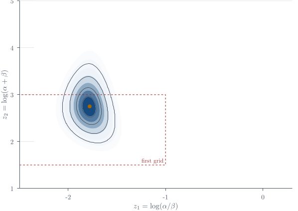
The binomial coefficient does not depend on (\alpha,\beta), so the hyperposterior kernel is \boxed{ p(\alpha,\beta\mid{\boldsymbol{y}}) \propto p(\alpha,\beta) \prod_{j=1}^J \frac{\Gamma(\alpha+\beta) \Gamma(y_j+\alpha) \Gamma(n_j-y_j+\beta)} {\Gamma(\alpha)\Gamma(\beta) \Gamma(n_j+\alpha+\beta)}}. This expression is available pointwise but is not a familiar normalised density.
Study-rate full conditional
Main article: Study-rate full conditional
Normalising gives \boxed{ \theta_j\mid\alpha,\beta,{\boldsymbol{y}} \sim\operatorname{Beta}(y_j+\alpha,n_j-y_j+\beta)}. Conditional on the hyperparameters, the study rates are independent, so the joint conditional is the product of these J Beta densities.
Examples
TG5 cattle hierarchy
Worked example from Hierarchical Bayes
A cattle-genetics meta-analysis illustrates hierarchical Bayes. The search was not exhaustive, but it recovered 14 independent studies, many of them unpublished, which produced 19 standardised estimates of a TG5 genotype effect on beef marbling. The studies covered four breed groups and four marbling measurements, so treating every estimate as an exchangeable replicate would erase scientifically meaningful structure.
The original study-level analyses compared the CC and TT genotypes with CT, then divided each contrast by its residual standard deviation. A schematic version of the hierarchy is \begin{align*} y_{ij}\mid\delta_i,w_{ij} &\sim\operatorname{N}(\delta_i,w_{ij}^{-1}),\\ \delta_i\mid\mu_{b(i)},\tau_{\mathrm{study}} &\sim\operatorname{N}(\mu_{b(i)},\tau_{\mathrm{study}}^{-1}),\\ \mu_b\mid\mu_0,\tau_{\mathrm{breed}} &\sim\operatorname{N}(\mu_0,\tau_{\mathrm{breed}}^{-1}),\\ \mu_0&\sim\operatorname{N}(0,\xi^2), \qquad \xi^2\text{ large}. \end{align*} Here w_{ij} records the within-study information, \delta_i is a study effect, and \mu_b is a breed-group effect. Precision parameters were given diffuse scaled inverse-\chi^2-type priors in the applied analysis. The diagrammatic flow is
\text{overall effect}\longrightarrow \text{breed effect}\longrightarrow \text{study effect}\longrightarrow \text{observed contrast}.
The hierarchy performs partial pooling at more than one level. The reported posterior for TT minus CC lay mostly above zero, with a smaller shift for one T copy, but the important methodological point is that every conclusion and every uncertainty interval came from one coherent multilevel fit. The example connects Bayesian random parameters to mixed models. The analysis was fitted in WinBUGS using a Gibbs sampler; the “GS” in the software name stands for Gibbs sampling.
Rat-tumour hierarchy
Worked example from Hierarchical Bayes
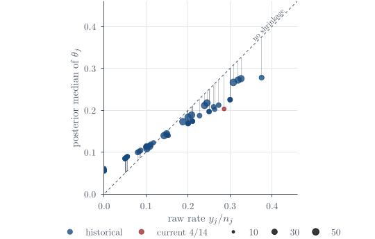
Tumour rates in female F344 rats supply a second hierarchical example. In a current control study, y=4 of n=14 rats developed one or more tumours over two years. A one-study model is
Y\mid\theta\sim\operatorname{Bin}(14,\theta), \qquad \theta\sim\operatorname{Beta}(\alpha,\beta),
giving
\theta\mid Y=4 \sim\operatorname{Beta}(\alpha+4,\beta+10).
The question is how to choose (\alpha,\beta) when 70 earlier control studies are available.
Let study j contribute y_j tumour-bearing rats from n_j animals. The hierarchical model is Y_j\mid\theta_j,n_j\sim\operatorname{Bin}(n_j,\theta_j), \qquad \theta_j\mid\alpha,\beta \stackrel{\mathrm{iid}}{\sim}\operatorname{Beta}(\alpha,\beta), \quad j=1,\ldots,J. Each study has its own rate, but all study rates are drawn from a common population distribution.
Q23. Rat-tumour studies and hierarchical shrinkage
Question page: Q23. Rat-tumour studies and hierarchical shrinkage
[12 marks]
Suppose J related studies record tumour counts Y_j\mid\theta_j\sim\operatorname{Binomial}(n_j,\theta_j), \qquad j=1,\ldots,J, independently conditional on the study rates. Assume \theta_j\mid\alpha,\beta \overset{\mathrm{iid}}{\sim}\operatorname{Beta}(\alpha,\beta), \qquad \alpha\sim\operatorname{Exp}(1),\quad \beta\sim\operatorname{Exp}(1), where the two hyperpriors are independent. Write \mathbf y=(y_1,\ldots,y_J); the sample sizes n_j are known. You may use B(a,b)=\int_0^1 t^{a-1}(1-t)^{b-1}\,dt, \qquad f(\theta\mid a,b)=\frac{\theta^{a-1}(1-\theta)^{b-1}}{B(a,b)}.
(a) [2 marks] Derive and identify the full conditional distribution \theta_j\mid\alpha,\beta,\mathbf y.
(b) [3 marks] For this part only, fix \alpha=2 and \beta=8. Two studies report (y_1,n_1)=(4,10),\qquad (y_2,n_2)=(40,100). Calculate both posterior means. Although both observed proportions equal 0.4, explain why the posterior means differ and identify which study experiences stronger shrinkage.
(c) [4 marks] Return to unknown \alpha,\beta. Integrate out the study rates to derive:
(i) the marginal probability \mathbb{P}(Y_j=y_j\mid\alpha,\beta);
(ii) the marginal posterior kernel p(\alpha,\beta\mid\mathbf y).
Express your answers using Beta functions. Explain why the Beta prior’s normalising factor cannot be discarded when deriving this hyperparameter posterior.
(d) [3 marks] Explain how the full Bayesian model allows studies to share information. What uncertainty is omitted if \alpha,\beta are instead estimated from the data and then treated as known?
Definitions. Study j has observed count y_j, known size n_j, and unknown rate \theta_j; \alpha,\beta>0 are shared hyperparameters. A \operatorname{Beta}(\alpha,\beta) density is \theta^{\alpha-1}(1-\theta)^{\beta-1}/B(\alpha,\beta) on (0,1), where B(a,b)=\int_0^1u^{a-1}(1-u)^{b-1}\,du. \operatorname{Exp}(1) uses rate one. Partial pooling allows different study rates linked through a common population distribution.
Assumptions. The hierarchy assumes conditional independence of studies given their rates, and iid Beta rates given \alpha,\beta. Thus its joint density factors as p(\alpha)p(\beta)\prod_jp(\theta_j\mid\alpha,\beta)p(y_j\mid\theta_j), with independent rate-one exponential hyperpriors. Only in part (b) are the hyperparameters fixed at the supplied values.
(a) Full conditional for a study rate. Holding \alpha,\beta fixed, the factors involving \theta_j are \begin{aligned} p(\theta_j\mid\alpha,\beta,\mathbf y) &\propto p(y_j\mid\theta_j)p(\theta_j\mid\alpha,\beta)\\ &\propto\theta_j^{y_j}(1-\theta_j)^{n_j-y_j} \theta_j^{\alpha-1}(1-\theta_j)^{\beta-1}\\ &=\theta_j^{\alpha+y_j-1}(1-\theta_j)^{\beta+n_j-y_j-1}. \end{aligned} Therefore \boxed{\theta_j\mid\alpha,\beta,\mathbf y \sim\operatorname{Beta}(\alpha+y_j,\beta+n_j-y_j),\qquad 0<\theta_j<1.} Conditional on the hyperparameters and data, the study rates are independent. Other studies’ observations affect this study’s marginal posterior through learning \alpha,\beta, not through an additional factor in this full conditional.
(b) Posterior means and shrinkage. For fixed \alpha=2, \beta=8, the population mean is \frac{\alpha}{\alpha+\beta}=\frac2{10}=0.2. The two posteriors are \theta_1\mid\alpha=2,\beta=8,\mathbf y\sim\operatorname{Beta}(6,14), \theta_2\mid\alpha=2,\beta=8,\mathbf y\sim\operatorname{Beta}(42,68). Thus their posterior means are \boxed{\mathbb{E}(\theta_1\mid\alpha=2,\beta=8,\mathbf y)=\frac6{20}=0.3,} \boxed{\mathbb{E}(\theta_2\mid\alpha=2,\beta=8,\mathbf y)=\frac{42}{110} \approx0.3818.} To see the shrinkage explicitly, write \frac{\alpha+y_j}{\alpha+\beta+n_j} =\frac{\alpha+\beta}{\alpha+\beta+n_j} \frac{\alpha}{\alpha+\beta} +\frac{n_j}{\alpha+\beta+n_j}\frac{y_j}{n_j}. Both sample proportions equal 0.4, but study 1 puts weight 10/20=1/2 on the population mean, whereas study 2 puts only 10/110=1/11 on it. The smaller study therefore experiences stronger shrinkage toward 0.2. The larger study has more information about its own rate, so its posterior mean remains closer to its observed proportion.
(c) Integrating out the study rates. For one study, retain the normalising factor of the Beta density: \begin{aligned} \mathbb{P}(Y_j=y_j\mid\alpha,\beta) &=\int_0^1 p(y_j\mid\theta_j)p(\theta_j\mid\alpha,\beta)\,d\theta_j\\ &=\binom{n_j}{y_j}\frac1{B(\alpha,\beta)} \int_0^1\theta_j^{y_j+\alpha-1} (1-\theta_j)^{n_j-y_j+\beta-1}\,d\theta_j\\ &=\boxed{\binom{n_j}{y_j} \frac{B(\alpha+y_j,\beta+n_j-y_j)}{B(\alpha,\beta)}.} \end{aligned} This is a Beta–Binomial marginal distribution, with y_j\in\{0,\ldots,n_j\}.
The independent rate-one exponential hyperpriors give p(\alpha,\beta)=e^{-\alpha-\beta},\qquad \alpha>0,\quad\beta>0. The studies remain independent conditional on the hyperparameters after their individual rates have been integrated out. Consequently, \begin{aligned} p(\alpha,\beta\mid\mathbf y) &\propto p(\alpha,\beta) \prod_{j=1}^{J}\mathbb{P}(Y_j=y_j\mid\alpha,\beta)\\ &\propto e^{-(\alpha+\beta)} \prod_{j=1}^{J} \frac{B(\alpha+y_j,\beta+n_j-y_j)}{B(\alpha,\beta)}. \end{aligned} Hence \boxed{ p(\alpha,\beta\mid\mathbf y) \propto e^{-(\alpha+\beta)}B(\alpha,\beta)^{-J} \prod_{j=1}^{J}B(\alpha+y_j,\beta+n_j-y_j), \quad \alpha,\beta>0. } The binomial coefficients can be dropped because the observed y_j and known n_j make them constant with respect to \alpha,\beta. However, 1/B(\alpha,\beta) depends on the hyperparameters, so it must remain. A factor constant in \theta_j need not be constant in \alpha,\beta.
(d) Sharing information and hyperparameter uncertainty. Every study contributes to the posterior for the common population parameters \alpha,\beta. That posterior then contributes to each study-specific posterior through p(\theta_j\mid\mathbf y) =\int_0^\infty\!\int_0^\infty p(\theta_j\mid\alpha,\beta,\mathbf y) p(\alpha,\beta\mid\mathbf y)\,d\alpha\,d\beta. This is partial pooling: study rates can differ, but they are connected by a population distribution learned from all the studies. The model does not force them to be identical, and it does not treat them as unrelated.
Replacing \alpha,\beta by fixed estimates is an empirical-Bayes plug-in analysis. It omits uncertainty about the population distribution’s parameters. For example, the law of total variance gives \begin{aligned} \operatorname{Var}(\theta_j\mid\mathbf y) ={}&\mathbb{E}\!\left[ \operatorname{Var}(\theta_j\mid\alpha,\beta,\mathbf y) \mid\mathbf y\right]\\ &+\operatorname{Var}\!\left[ \mathbb{E}(\theta_j\mid\alpha,\beta,\mathbf y) \mid\mathbf y\right]. \end{aligned} The second term represents variation in the conditional mean as the hyperparameters vary under their posterior. A plug-in calculation does not propagate this variation and can therefore give an overly precise account of uncertainty.
Key result. Conditional conjugacy does not eliminate uncertainty in the hyperparameters. Full Bayes learns their distribution and averages over it.
Question 17. Hierarchical Poisson model
Question page: Question 17. Hierarchical Poisson model
Suppose J factories manufacture components. Factory j produces n_j observations of the number of defective components per batch.
Assume
Y_{ij}\mid\theta_j\stackrel{\mathrm{ind}}{\sim}\operatorname{Poisson}(\theta_j), \qquad i=1,\ldots,n_j,\quad j=1,\ldots,J.
Here, \theta_j>0 represents the expected number of defects per batch in factory j.
Rather than modelling the factory rates independently, we assume
\theta_j\mid\lambda\overset{\text{iid}}{\sim}\operatorname{Gamma}(a,\lambda),
where a>0 is known and \lambda>0 is an unknown common hyperparameter.
Finally, assign the hyperprior
\lambda\sim\operatorname{Gamma}(c,d),
where c,d>0 are known.
All Gamma distributions use the shape–rate parameterisation:
f(x\mid a,b)=\frac{b^{a}}{\Gamma(a)}x^{a-1}e^{-bx}, \qquad x>0.
(a) Write down the joint density p({\boldsymbol{Y}},{\boldsymbol{\theta}},\lambda) up to proportionality in the unknown parameters.
(b) Derive the full conditional distribution p(\theta_j\mid\lambda,{\boldsymbol{Y}}) for each factory j. Identify its distribution and parameters.
(c) Derive the full conditional distribution p(\lambda\mid{\boldsymbol{\theta}},{\boldsymbol{Y}}). Identify its distribution and parameters.
(d) Using your results from (b) and (c), describe a Gibbs sampling algorithm targeting p({\boldsymbol{\theta}},\lambda\mid{\boldsymbol{Y}}).
(e) Explain how the hierarchical model allows observations from one factory to influence inference about another factory’s defect rate.
Definitions. Y_{ij} is the count from batch i in factory j, \theta_j is that factory’s mean count, and \lambda is a shared unknown gamma rate. The known shape is a, while c,d define the shape–rate gamma hyperprior on \lambda. Write s_j=\sum_iY_{ij} and \bar Y_j=s_j/n_j. The conditional hierarchy is \lambda\longrightarrow{\boldsymbol{\theta}}\longrightarrow{\boldsymbol{Y}}.
(a) Let s_j=\sum_{i=1}^{n_j}Y_{ij}. Since {\boldsymbol{Y}}\perp\lambda\mid{\boldsymbol{\theta}},
p({\boldsymbol{Y}},{\boldsymbol{\theta}},\lambda) = p({\boldsymbol{Y}}\mid{\boldsymbol{\theta}})\,p({\boldsymbol{\theta}}\mid\lambda)\,p(\lambda).
For \theta_j>0 and \lambda>0,
\begin{aligned} p({\boldsymbol{Y}}\mid{\boldsymbol{\theta}}) &= \Biggl(\prod_{j=1}^{J}\prod_{i=1}^{n_j}\frac{1}{Y_{ij}!}\Biggr) \prod_{j=1}^{J}e^{-n_j\theta_j}\theta_j^{s_j},\\ p({\boldsymbol{\theta}}\mid\lambda) &= \Biggl(\frac{\lambda^{a}}{\Gamma(a)}\Biggr)^{J} \prod_{j=1}^{J}\theta_j^{a-1}e^{-\lambda\theta_j},\\ p(\lambda) &= \frac{d^{c}}{\Gamma(c)}\lambda^{c-1}e^{-d\lambda}. \end{aligned}
The factors 1/Y_{ij}!, \Gamma(a)^{-J} and d^{c}/\Gamma(c) do not depend on ({\boldsymbol{\theta}},\lambda). Dropping them leaves
\boxed{ p({\boldsymbol{Y}},{\boldsymbol{\theta}},\lambda) \propto \lambda^{aJ+c-1}e^{-d\lambda} \prod_{j=1}^{J} \theta_j^{s_j+a-1}e^{-(n_j+\lambda)\theta_j}. }
(b) In the kernel from (a), the factors containing \theta_j are
\theta_j^{s_j+a-1}e^{-(n_j+\lambda)\theta_j} = \theta_j^{(s_j+a)-1}e^{-(n_j+\lambda)\theta_j}, \qquad\theta_j>0.
No other rate appears. Here s_j+a>0 because a>0 and s_j\ge 0, and n_j+\lambda>0 because \lambda>0. This is a shape–rate gamma kernel, so
\boxed{ \theta_j\mid\lambda,{\boldsymbol{Y}} \sim \operatorname{Gamma}\!\left(a+\sum_{i=1}^{n_j}Y_{ij},\ n_j+\lambda\right). }
(c) In the kernel from (a), the factors containing \lambda are
\lambda^{aJ+c-1} \exp\Bigl(-\lambda\sum_{j=1}^{J}\theta_j\Bigr)e^{-d\lambda} = \lambda^{(aJ+c)-1} \exp\Bigl(-\Bigl(d+\sum_{j=1}^{J}\theta_j\Bigr)\lambda\Bigr),
for \lambda>0. Given {\boldsymbol{\theta}}, the observations do not appear. The shape aJ+c>0, and the rate d+\sum_j\theta_j>0 because d>0. Thus
\boxed{ \lambda\mid{\boldsymbol{\theta}},{\boldsymbol{Y}} \sim \operatorname{Gamma}\!\left(c+aJ,\ d+\sum_{j=1}^{J}\theta_j\right). }
(d) By (b) and (c), alternate a block of factory-rate draws with a shared-rate draw. Recall s_j=\sum_iY_{ij}.
All gamma distributions in the algorithm use rates. The J factory draws are conditionally independent given the previous \lambda, so their order does not matter. The final draw uses all newly updated rates. These exact full-conditional updates preserve p({\boldsymbol{\theta}},\lambda\mid{\boldsymbol{Y}}); assess convergence and mixing before using the retained output.
(e) By (b), \theta_j depends on the other factories only through \lambda. Counts from factory k update \theta_k, and by (c) every rate enters the conditional distribution of the shared \lambda. That \lambda is the second parameter of \theta_j. This dependence through the common hyperparameter is borrowing strength: observations from one factory inform the defect rate at another.
At a fixed \lambda, the conditional posterior mean makes the shrinkage explicit:
\mathbb{E}(\theta_j\mid\lambda,{\boldsymbol{Y}}) =\frac{s_j+a}{n_j+\lambda} =\frac{n_j}{n_j+\lambda}\bar Y_j +\frac{\lambda}{n_j+\lambda}\frac a\lambda.
This averages factory j’s sample mean and the common prior mean a/\lambda. For a given \lambda, smaller factories receive more pooling. The marginal posterior mean averages this expression over p(\lambda\mid{\boldsymbol{Y}}), which is informed by all factories. Fixing \lambda externally removes this route for other factories’ data to influence \theta_j. Integrating over a shared uncertain \lambda also generally makes the factory rates dependent in the joint posterior.
Figures
Used in
- Taught in Hierarchical Bayes, where the derivation and examples are.
- Also used in Exponential families and conjugacy · How to use the final preparation · Reference formulas and problem-solving workflow
- Questions that use it (2) — Question 17 · C9
- All 9 questions on Hierarchical Bayes
See also
Hyperparameter · Normal hierarchical shrinkage · Exchangeability · Empirical Bayes · Study-rate full conditional · Marginal hyperposterior · Uniformity depends on a domain · Grid Monte Carlo approximation