Limit theorems
Section of Functions of random variables and limit theorems, part of Probability
Limit theorems
| Type | Section |
| Taught in | Functions of random variables and limit theorems |
| Part | Probability |
| Questions using it | 2 |
Let X_1,X_2,\ldots be independent, identically distributed, with \mathbb{E} X_i=\mu, and write S_n=X_1+\cdots+X_n.
Theorem 1 (Law of large numbers) If the mean \mu exists, the strong law says
\mathbb{P}\Bigl(\lim_{n\to\infty} S_n/n=\mu\Bigr)=1.
If in addition the variance is finite, the weak law says that for every \varepsilon>0,
\lim_{n\to\infty}\mathbb{P}\bigl(|S_n/n-\mu|>\varepsilon\bigr)=0.
The weak law under a finite variance follows from Chebyshev’s inequality: \mathbb{P}(|S_n/n-\mu|>\varepsilon)\le \operatorname{Var}(S_n/n)/\varepsilon^2=\operatorname{Var}(X_1)/(n\varepsilon^2), which tends to zero.
The sample average converges to the expectation. That is the justification for estimating an unknown mean by the average of repeated measurements, and for reading a long-run relative frequency as a probability. The weak law says the probability of a large error disappears. The strong law says the error itself disappears, except on a set of outcomes of probability zero.
Chebyshev’s inequality, used above, is the general bound \mathbb{P}(|X-\mathbb{E} X|\ge \varepsilon)\le \operatorname{Var}(X)/\varepsilon^2, and Markov’s inequality is \mathbb{P}(X\ge x)\le \mathbb{E} X/x for a non-negative X and x>0.
Theorem 2 (Central limit theorem) If the X_i are independent and identically distributed with mean \mu and variance \sigma^2\in(0,\infty), then for every x
\lim_{n\to\infty}\mathbb{P}\Bigl(\frac{S_n-n\mu}{\sigma\sqrt{n}}\le x\Bigr)=\Phi(x),
where \Phi is the standard normal distribution function.
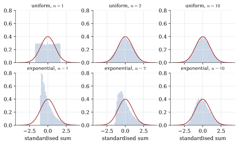
The shape of the parent distribution washes out of the centred and scaled sum. What remains is the standard normal distribution. For large n, S_n is approximately \operatorname{N}(n\mu, n\sigma^2), and the sample average is approximately \operatorname{N}(\mu,\sigma^2/n).
A binomial count X\sim\operatorname{Bin}(n,p) is a sum of n Bernoulli trials, so for large n
\mathbb{P}(X\le k)\approx \Phi\Bigl(\frac{k-np}{\sqrt{np(1-p)}}\Bigr).
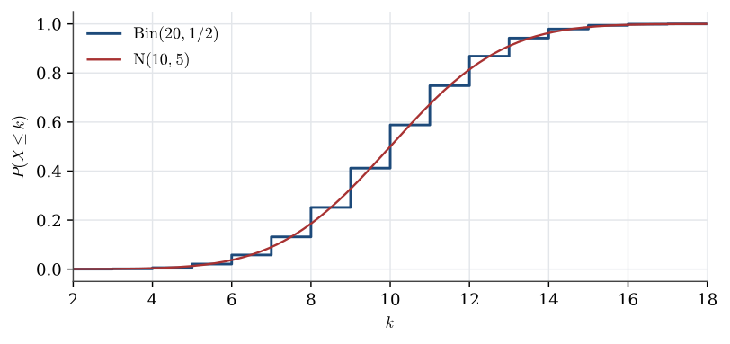
Example 1 (Normal approximation to a binomial) Let X\sim\operatorname{Bin}(20,1/2).
Question. Approximate \mathbb{P}(X\le8) by the central limit theorem, with and without a continuity correction, and compare with the exact value.
Solution. Here np=10 and np(1-p)=5. The exact probability is 0.2517. The plain approximation gives
\mathbb{P}(X\le8)\approx\Phi\Bigl(\frac{8-10}{\sqrt5}\Bigr)=\Phi(-0.894)=0.186,
which is poor. X is integer-valued, so \mathbb{P}(X\le8)=\mathbb{P}(X\le8.5), and the normal curve should be read at the midpoint between 8 and 9:
\mathbb{P}(X\le8)\approx\Phi\Bigl(\frac{8.5-10}{\sqrt5}\Bigr)=\Phi(-0.671)=0.251,
almost exact. A usual rule of thumb asks for both np and n(1-p) to be above 5.
The same approximation, applied to a sum of independent uniforms or to a sum of independent exponential variables, is how a probability about an average is evaluated when the exact distribution is awkward. The distribution function \Phi is the one attached to the normal law on the common distributions page.
Monotone maps change the density by the derivative of the inverse. Smooth maps in several dimensions change it by the absolute value of the Jacobian. Averages of independent copies converge to the mean, and the scaled fluctuation converges to a standard normal variable.
Used in
- Taught in Functions of random variables and limit theorems
- Also used in Hypothesis tests · Estimation examples · Chi-squared examples
- Questions that use it (2) — A normal approximation on an interval (answer) · A sieve for blueberries (answer)
- All 21 questions on Functions of random variables and limit theorems
See also
Transformation rule · Multivariate normal distribution · Affine images of normal vectors · Normal linear model · Law of large numbers · Central limit theorem · Distribution of a function or a sum · Jointly normal variables