Link function
Topic of Introduction to generalised linear models, part of Generalised linear models · Also in Introduction to generalised linear models, Underdispersion, positive responses, and quasi-likelihood
Link function
| Type | Topic |
| Taught in | Introduction to generalised linear models · Introduction to generalised linear models · Underdispersion, positive responses, and quasi-likelihood |
| Part | Generalised linear models |
| Questions using it | 5 |
The function g that ties the mean of a GLM to its linear predictor, g(\mu_i)=\mathbf{X}_i^\top\boldsymbol{\beta}. It is chosen so that every value of the linear predictor gives a legal mean: the logit keeps a probability in (0,1), the log keeps a count’s mean positive.
In Introduction to generalised linear models
Definition 1 Observations Y_1,\ldots,Y_n follow a generalised linear model when all three of the following are specified.
- Random component. The Y_i are independent, and each belongs to the same exponential family. The functions a, b, c, d and e are common; the parameter \theta_i may depend on i.
- Linear predictor. Covariate vectors {\boldsymbol{X}}_1,\ldots,{\boldsymbol{X}}_n and a coefficient vector \boldsymbol{\beta}=(\beta_0,\ldots,\beta_d)^\top form \eta_i={\boldsymbol{X}}_i^\top\boldsymbol{\beta}.
- Link. A monotone function g connects the mean \mu_i=\mathrm{E}(Y_i) to that predictor, g(\mu_i)={\boldsymbol{X}}_i^\top\boldsymbol{\beta}.
The three choices are separate, and all three are yours. You choose the distribution. You choose which covariates go into {\boldsymbol{X}}_i, and whether to transform them first: log dose is still just a column of {\color{blue}\boldsymbol{X}}. You choose the link. Nothing forces the link that is “canonical” for the distribution you chose.
Definition 2 The link g is canonical when the linear predictor is the natural parameter of the family: g(\mu_i)=b(\theta_i), in the notation of Equation (6) in Introduction to generalised linear models.
For the families above, the canonical links are
- normal: g(\mu)=\mu, the identity, because the natural parameter is the mean;
- Poisson: g(\mu)=\log\mu, because the natural parameter is \log\lambda and \mu=\lambda;
- binomial, including Bernoulli: g(\mu)=\log\{\mu/(1-\mu)\}, the logit;
- gamma, in the shape-and-rate form with mean \mu: g(\mu)=1/\mu, the inverse link.
If you call glm in R and name the family but not the link, you get the canonical link. That is a software default, not a scientific one. The canonical link for the gamma is the inverse link. The link used most often here for a positive continuous response is still the log link, because a slope is then a multiplicative change in the mean, and that is a sentence one can say to a collaborator. Canonical links are the natural mathematical choice. They are not always the appropriate one. You override the default by stating the link yourself.
The normal linear model is the GLM with identity link and normal random component: \mu_i={\boldsymbol{X}}_i^\top\boldsymbol{\beta} and \mathrm{Var}(Y_i)=\sigma^2. Logistic regression is the GLM with Bernoulli random component and the logit link Equation (5) in Introduction to generalised linear models. Writing those two out is not a new model. It is the definition, specialised.
A GLM is an exponential family, a linear predictor, and a link, chosen independently. The canonical link equates the linear predictor with the natural parameter. It is the default in R. It is not a requirement.
In Introduction to generalised linear models, continued
The logistic link is Equation (5) in Introduction to generalised linear models. It is the link we will interpret, and it is the canonical link.
The probit link replaces the logistic curve by a standard normal distribution function. If \Phi is the cumulative distribution function of \mathrm{N}(0,1), \Phi^{-1}(p_i)={\boldsymbol{X}}_i^\top\boldsymbol{\beta} \qquad\text{equivalently}\qquad p_i=\Phi({\boldsymbol{X}}_i^\top\boldsymbol{\beta}). Read it as a quantile. Compute {\boldsymbol{X}}_i^\top\boldsymbol{\beta}, find that point on the standard normal axis, and take the probability to its left. That left-tail probability is p_i. Any other continuous distribution function would give a link of the same type. The normal is the default.
The complementary log-log link is \log\bigl(-\log(1-p_i)\bigr)={\boldsymbol{X}}_i^\top\boldsymbol{\beta} \qquad\text{equivalently}\qquad p_i=1-\exp\bigl\{-\exp({\boldsymbol{X}}_i^\top\boldsymbol{\beta})\bigr\}. The exercise asks you to check that the right-hand side lies in (0,1) for every real linear predictor. This link is the one that does not treat the two tails symmetrically. Logit and probit both approach 0 and 1 in the same fashion, one a mirror of the other. Complementary log-log can stay near zero for longer and then rise more sharply towards one, or the reverse, depending on the sign of the slope. Use it when that asymmetry is the scientific point. Do not use it because you want a sentence about odds. The coefficient is a log-hazard, an instantaneous risk, and a hazard is much harder to explain to a medical collaborator than an odds ratio.
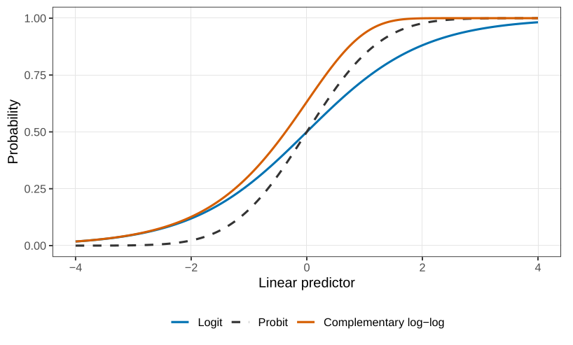
In Figure the logit and the probit differ in the tails and agree through the middle. In a fitted model they almost always agree, close enough that the two curves will not separate. A probit essentially never has to be the link reported to an applied scientist. A log-odds can be explained. A computer scientist or an engineer will sometimes prefer the probit, because a normal quantile is already their language. When there is a choice, and the person across the table is not one of those, use the logit. Goodness of fit will not be the reason to switch.
In Underdispersion, positive responses, and quasi-likelihood
A clotting time, or an insurance claim amount, is continuous and cannot be negative. Three links are in ordinary use: \begin{align*} \log\mu_i&={\boldsymbol{X}}_i^\top\boldsymbol{\beta}, & \mu_i&=\exp({\boldsymbol{X}}_i^\top\boldsymbol{\beta}),\\ \mu_i^{-1}&={\boldsymbol{X}}_i^\top\boldsymbol{\beta}, & \mu_i&=1/({\boldsymbol{X}}_i^\top\boldsymbol{\beta}),\\ \mu_i^{-2}&={\boldsymbol{X}}_i^\top\boldsymbol{\beta}, & \mu_i&=1/\sqrt{{\boldsymbol{X}}_i^\top\boldsymbol{\beta}}. \end{align*} The log link is the one with a direct reading, and it keeps \mu positive for every finite predictor. It is not the canonical link for the gamma or the inverse Gaussian, so R will not choose it unless you name it. The canonical link for the gamma is the inverse link. The canonical link for the inverse Gaussian is the inverse quadratic. Both of those are only positive when {\boldsymbol{X}}^\top\boldsymbol{\beta}>0. If the linear predictor changes sign, the inverse link produces a negative mean, and the square root in the inverse quadratic leaves the reals. It is sometimes said that the inverse quadratic “ensures” non-negativity because a complex mean is not a mean. That is a restriction on the domain of \boldsymbol{\beta}, not a guarantee for every coefficient vector. You still have to keep the linear predictor positive.
Used in
- Taught in Introduction to generalised linear models · Introduction to generalised linear models · Underdispersion, positive responses, and quasi-likelihood
- Questions that use it (5) — Q36 (answer) · Q38 (answer) · Q57 · Question 21 (answer) · C17
- All 9 questions on Introduction to generalised linear models
See also
Generalised linear model · Linear predictor · Three components of a GLM · Logit link · Exponential family · Mean and variance of an exponential family · Canonical link · What a regression statement is hiding