Ingredients of a hypothesis test
Section of Hypothesis tests, part of Statistical inference
Ingredients of a hypothesis test
| Type | Section |
| Taught in | Hypothesis tests |
| Part | Statistical inference |
The model is a random sample, or a count, whose distribution depends on \theta. The model must leave \theta free. In the blood-pressure example the model is X_i independent \operatorname{N}(\mu,7^2) with \mu unknown; setting \mu=127 in the model would assume the answer.
Definition 1 (Null and alternative hypotheses) The null hypothesis H_0 and the alternative hypothesis H_1 are two disjoint statements about the parameter, H_0:\theta\in\Theta_0 and H_1:\theta\in\Theta_1. H_0 is the statement being tested, often a single value \theta_0. H_1 is the claim the test is trying to detect.
The null is rejected only on strong evidence, so the claim of interest goes in the alternative. For the blood pressures, H_0:\mu=127 against H_1:\mu\neq127. For the serves, H_0:p=0.6 against H_1:p>0.6. An alternative of the form \theta\neq\theta_0 is two-sided; \theta>\theta_0 and \theta<\theta_0 are one-sided.
A test statistic T is a statistic that is sensitive to the difference between H_0 and H_1. Like any statistic, it must not contain unknown parameters. Its null distribution is the distribution of T when H_0 is true. In the blood-pressure example \overline X, \overline X-127 and \sum X_i all work, because each carries the same information and each has a known null distribution.
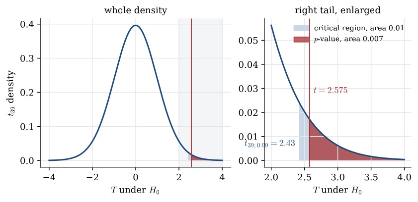
Definition 2 (Critical region) A critical region C is a set of values of the test statistic. The test rejects H_0 when T\in C. A right-sided region is [c,\infty), a left-sided region is (-\infty,c], and a two-sided region is (-\infty,c_1]\cup[c_2,\infty).
The shape of C follows from H_1. For the blood pressures, a mean much larger or much smaller than 127 is evidence against H_0, so C is two-sided. For the serves, only a large count is evidence for improvement, so C=\{c,\ldots,15\}.
Definition 3 (p-value) The p-value of an observed statistic t is the probability, under H_0, that T is at least as extreme as t, in the direction of H_1. For a two-sided normal or t statistic it is twice the one-sided tail probability beyond |t|.
Concretely, for a left-sided test p=\mathbb{P}_{H_0}(T\le t), for a right-sided test p=\mathbb{P}_{H_0}(T\ge t), and for a two-sided test
p=\min\{2\mathbb{P}_{H_0}(T\le t),\ 2\mathbb{P}_{H_0}(T\ge t)\}.
The doubling matters. The diabetics question was whether they differ, in either direction, so the extreme event is \{\overline X\ge130\}\cup\{\overline X\le124\}, and the p-value is 2\times8.3\times10^{-6}=1.7\times10^{-5}. The single tail is the p-value for the different question of whether diabetic men have higher blood pressure.
A small p-value is stronger evidence against H_0 than a large one. Conventional markers are 0.10 for suggestive evidence, 0.05 for reasonable evidence and 0.01 for strong evidence. They are conventions about long-run error rates, not probabilities that the decision is correct. How much evidence is enough depends on what the decision costs: a conviction for a serious crime needs more than a parking fine.
Used in
See also
Null and alternative hypotheses · Critical region · p-value · Type I and type II errors · Neyman–Pearson approach · Power function · One-sample t test · Two-sample t test