Gibbs sampling
Section of Markov chains, Gibbs sampling, and Metropolis–Hastings, part of Bayesian statistics
Gibbs sampling
| Type | Section |
| Taught in | Markov chains, Gibbs sampling, and Metropolis–Hastings |
| Part | Bayesian statistics |
| Questions using it | 18 |
Definition 1 (Systematic-scan Gibbs sampler) Suppose the target is a joint density \pi(x_1,\ldots,x_p) that is difficult to sample from directly, while every full conditional is available. One Gibbs sweep updates coordinates in order: \begin{align*} X_1^{(t+1)}&\sim \pi(x_1\mid X_2^{(t)},\ldots,X_p^{(t)}),\\ X_2^{(t+1)}&\sim \pi(x_2\mid X_1^{(t+1)},X_3^{(t)},\ldots,X_p^{(t)}),\\ &\ \vdots\\ X_p^{(t+1)}&\sim \pi(x_p\mid X_1^{(t+1)},\ldots,X_{p-1}^{(t+1)}). \end{align*} Each update uses the newest available coordinate values. Under standard ergodicity conditions, X^{(t)} converges in distribution to \pi. For a full conditional, the other coordinates are held fixed. Therefore
\pi(x_i\mid x_{-i}) =\frac{\pi(x_i,x_{-i})}{\pi(x_{-i})} \propto\pi(x_i,x_{-i}) \quad\text{as a function of }x_i.
Terms involving only x_{-i} may be dropped, but any term that still contains x_i must remain. Gibbs accepts every coordinate draw because it samples from the exact conditional rather than proposing and rejecting a candidate.
Bivariate exponential example
Main article: Bivariate exponential example
Example 1 (Bivariate exponential target) The target is
\pi(x_1,x_2)\propto e^{-x_1x_2-x_1-x_2}, \qquad x_1,x_2\geq0.
Question. Derive both full conditional distributions and use them to specify a systematic-scan Gibbs sampler.
Solution. To obtain X_1\mid X_2=x_2, hold x_2 fixed: \begin{align*} \pi(x_1\mid x_2) &\propto\pi(x_1,x_2)\\ &\propto e^{-x_1x_2-x_1-x_2}\\ &\propto e^{-x_1(x_2+1)}, \qquad x_1\geq0. \end{align*} The omitted factor e^{-x_2} is constant in x_1. Normalising gives
\pi(x_1\mid x_2)=(x_2+1)e^{-(x_2+1)x_1},
so
X_1\mid X_2=x_2\sim\operatorname{Exp}(x_2+1).
By symmetry,
X_2\mid X_1=x_1\sim\operatorname{Exp}(x_1+1).
Starting from any nonnegative pair (x_1^{(0)},x_2^{(0)}), the sampler is \begin{align*} x_1^{(t+1)}&\sim\operatorname{Exp}(x_2^{(t)}+1),\\ x_2^{(t+1)}&\sim\operatorname{Exp}(x_1^{(t+1)}+1). \end{align*}
Running the Gibbs sampler
Main article: Running the Gibbs sampler
The full conditionals above are the part to derive. Once they are correct, the sampler itself is a short computation. The newest value of x_1 must be used in the update of x_2; using the old value in both lines would define a different transition rule.
gibbs_exp <- function(iterations) {
  out <- matrix(0, iterations, 2)  # start at (0, 0)
  for (t in 2:iterations) {
    out[t, 1] <- rexp(1, rate = out[t - 1, 2] + 1)
    out[t, 2] <- rexp(1, rate = out[t, 1] + 1)
  }
  out
}
set.seed(3500)
draw <- gibbs_exp(20000)
keep <- draw[-seq_len(1000), ]
matplot(keep, type = "l", lty = 1)
acf(keep[, 1])
The trace plot and autocorrelation function are not substitutes for the stationarity argument. They address the separate practical question of whether this finite run appears to have explored the target well enough for the posterior summary at hand.
Normal mean and variance example
Main article: Gibbs sampler for a normal mean and variance
Example 2 (Normal mean and variance) Question. For the joint normal-model posterior in Equation (4) in Conjugate analysis for normal models, describe a systematic Gibbs sampler and state how retained draws estimate the posterior mean of \mu.
Solution. For the joint posterior in Equation (4) in Conjugate analysis for normal models, alternate \begin{align*} \mu^{(t+1)}&\sim p(\mu\mid\sigma^{2(t)},{\boldsymbol{x}}) \quad\text{using (5)},\\ \sigma^{2(t+1)}&\sim p(\sigma^2\mid\mu^{(t+1)},{\boldsymbol{x}}) \quad\text{using (6)}. \end{align*} After discarding a warm-up segment, Monte Carlo estimates use the retained draws. For example,
\widehat{\mathbb{E}}(\mu\mid{\boldsymbol{x}}) =\frac1L\sum_{t=B+1}^{B+L}\mu^{(t)},
where B is the number of discarded iterations. Because the draws are dependent, L correlated draws contain less information than L independent draws. Autocorrelation, trace plots, multiple chains, and effective sample size are therefore part of a serious analysis.
Initialisation, warm-up, and dependence
Main article: Initialisation, warm-up, and dependence
Remark 1 (Warm-up is not a convergence proof). The chain should be initialised in a plausible region when one is available. A start many standard deviations from the typical set can require a long time to return, while a start at the mean of a separated mixture can lie in a low-density gap. Multiple dispersed chains help reveal failure to explore all modes; they do not repair it automatically.
Discarding early draws is called warm-up or burn-in. It limits dependence on the chosen initial state, but it is not a proof of convergence. Strong posterior correlation produces staircase-like Gibbs paths and high autocorrelation. Separated modes are harder still because a coordinate-wise move may have to cross a low-density barrier.
Thinning by retaining every kth draw reduces storage and visible serial dependence, but usually throws away usable information. Unless storage or an expensive downstream calculation is the constraint, retain all post-warm-up draws and quantify their effective sample size. Posterior means, probabilities, and equal-tailed intervals are computed from those draws; a continuous MAP is found by optimisation, not by asking which simulated value occurred most often.
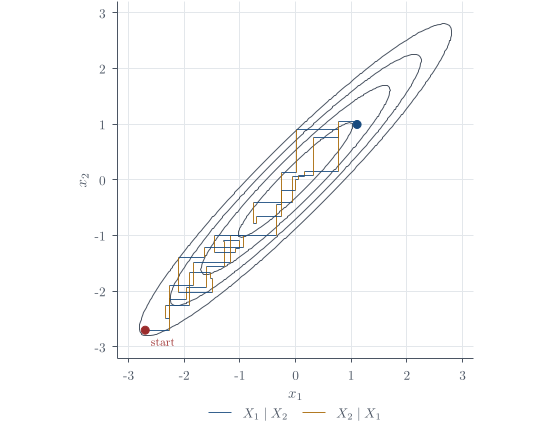
Burn-in is a practical attempt to reduce the memory of a poor starting point; it is not a theorem that the retained chain has converged. A very long run can make an initial mistake negligible, but separated modes may still defeat a sampler that never travels between them. The central question is not merely how many iterations were produced, but whether the chain explored every region whose posterior mass matters often enough to estimate their relative weights.
The deliberately absurd comparison is between 100{,}000 draws and 100 billion draws. A fixed number of poor initial draws becomes negligible as a proportion of an enormous run. That arithmetic does not help if an important remote mode is never visited: the question is whether such a region would appear in a run of that length, not merely whether the denominator is large.
Raising a target density to a power, \pi(x)^c, sharpens it for c>1 and flattens it for 0<c<1. Simulated annealing gradually changes such a power or temperature so that sampling increasingly resembles optimisation.
Used in
- Taught in Markov chains, Gibbs sampling, and Metropolis–Hastings
- Also used in Markov chains · Conjugate analysis for normal models · Exponential families and conjugacy · Hierarchical Bayes · Bayesian linear regression · Reference formulas and problem-solving workflow
- Questions that use it (18) — A bivariate-normal Gibbs sampler · Q4 · Q9 · Q18 · Q25 · Q26 · Q43 · Q51 · Q58 · Q59 · Question 3 · Question 6 · Question 9 · Question 12 (answer) · Question 13 · Question 16 · Question 17 · C13
- All 31 questions on Markov chains, Gibbs sampling, and Metropolis–Hastings
See also
Systematic-scan Gibbs sampler · Full conditional distribution · Three easy confusions · Markov chain · Stationarity and detailed balance · Detailed balance implies stationarity · Warm-up is not a convergence proof · Metropolis–Hastings update